How to Export Gerber Files from KiCad for PCB Manufacturing?

September 22nd, 2026

Here is how to export Gerber files from KiCad for manufacturing: create one Gerber file for each required PCB layer and separate drill files for holes and slots. Most fabricators expect both sets in one ZIP. Gerbers without drill data omit the hole pattern, while a native KiCad board file leaves the final plot choices to someone else.

The instructions match KiCad 10 and follow the files from the saved board through GerbView and into a revision-controlled ZIP. Older releases may label the menu differently, although File > Plot opens the plotting dialog in many earlier versions.

How to export Gerber files from KiCad, PCB design layers and fabrication output on an engineering workstation

What Should You Check Before Exporting Gerber Files from KiCad?

Check the KiCad source design before creating manufacturing files. The plotter reproduces the board as it exists; it does not repair an open outline, an unconnected net, an omitted layer, or an outdated copper-zone fill. Open the final production revision in PCB Editor and save it before running the checks.

Run the Design Rules Checker: Use Inspect > Design Rules Checker and review violations, unconnected items, and schematic-to-PCB differences. Resolve real problems and document any deliberate exclusions instead of assuming the fabricator will interpret them.
Validate Edge.Cuts: Confirm that the external outline is one closed, non-self-intersecting shape and that intended internal cutouts are also closed. KiCad shades a valid closed board area and reports malformed outlines through DRC.
Confirm the copper stack: Verify the enabled copper-layer count and order in Board Setup. A 4-layer board must have the correct internal layers and stack sequence before those layers are plotted.
Review mask and silkscreen: Check mask openings around pads and make sure silkscreen text and graphics do not cover exposed solderable areas. Remove information that does not belong on the manufactured board.
Inspect drilled features: Review plated through holes, non-plated holes, slots, and mounting holes. Confirm that each feature has the intended plating property and finished purpose.
Refill copper zones: Press B or use the zone-fill command, then save the board. Enabling KiCad’s plot-time zone check provides another safeguard, but the source board should already be current.

This preflight checks the editable design. It does not replace the later Gerber review, which checks the actual files that will leave your computer.

How to Export Gerber Files from KiCad Step by Step?

Use PCB Editor to export Gerber files from KiCad into a clean revision folder, then inspect what KiCad actually wrote. Each step below keeps the output tied to the same saved board revision and ends with something you can check.

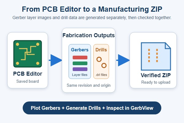
How to export Gerber files from KiCad, process from PCB Editor through separate Gerber and drill output to a verified ZIP

Open the final board in PCB Editor: Confirm the project name and revision, save the .kicad_pcb file, and make sure the canvas shows the board you intend to order.
Open the Gerber dialog: Choose File > Fabrication Outputs > Gerbers (.gbr). File > Plot opens the same dialog when Gerber is selected as the plot format. The Plot window should show the board’s enabled layer list.
Choose a dedicated output folder: Use a new folder such as fabrication/rev-b/gerber. It should not contain files from an earlier revision. The output path displayed in the dialog should point to that folder.
Select the required layers: Include every copper layer used by the design, the top and bottom solder-mask layers, any silkscreen layers that contain board markings, and Edge.Cuts. Add paste layers only when the package also serves a stencil or assembly workflow.
Set the relevant plot options: Keep the drawing sheet out of the Gerbers, keep the plot at its real scale, use a consistent origin, and enable the zone-fill check. Change compatibility options only when your manufacturer provides a requirement.
Click Plot: KiCad writes one Gerber file for each selected layer. Review the Output Messages panel and open the destination folder. You should see a fresh set whose timestamps match this export.

Do not ZIP the folder yet. First confirm the layer set, generate the drill output, and inspect both together.

Which Gerber Layers Should You Export for PCB Manufacturing?

A bare PCB package normally includes every used copper layer, both solder-mask layers, the required silkscreen layers, and Edge.Cuts. The exact count changes with the board stack and whether artwork exists on the back. The table separates bare-board files from stencil or assembly outputs.

Layer	Purpose and Export Rule
F.Cu	Front copper image; always export it when the board uses front copper.
B.Cu	Back copper image; always export it for a 2-layer or multilayer board.
In1.Cu, In2.Cu, and other internal copper	Inner signal or plane layers; export every enabled internal layer in the correct stack order.
F.Mask	Front solder-mask openings; normally required.
B.Mask	Back solder-mask openings; normally required.
F.Silkscreen	Front legend and reference markings; export when used.
B.Silkscreen	Back legend and reference markings; export when used.
Edge.Cuts	External profile and internal cutouts; required for the manufactured board shape.
F.Paste and B.Paste	Solder-paste stencil apertures; use for stencil or assembly preparation, not normally for bare-board fabrication.
F.Fab and B.Fab	Assembly and fabrication drawing detail; send separately when requested and never substitute it for copper or Edge.Cuts.

For a typical 2-layer bare board, the practical minimum is F.Cu, B.Cu, F.Mask, B.Mask, Edge.Cuts, the silkscreen layers that contain artwork, and the drill file or files. For a multilayer design, add every internal copper layer and provide the intended stackup separately so the manufacturer can map the layer order without guessing.

Which KiCad Gerber Plot Settings Matter for PCB Manufacturing?

Keep the defaults that preserve 1:1 geometry, then change only options that affect file interpretation or compatibility. KiCad exposes many plot controls because the same dialog can also create PDF, SVG, DXF, and other outputs. A Gerber handoff uses a smaller, more focused subset.

Plot drawing sheet: off: The page border and title block are document furniture, not the PCB profile. Edge.Cuts should carry the board shape.
Check zone fills before plotting: on: KiCad warns that plot output can be wrong when outdated zones are not checked and refilled.
Plot on all layers: normally empty: This feature overlays selected items onto every base layer. Use it only for a deliberate documentation requirement, not to place Edge.Cuts or silkscreen into every Gerber by habit.
Gerber X2: use when accepted: X2 adds file-function, net, and other attributes that can help CAM interpretation. Turn it off only when a manufacturer reports that its older CAM system cannot process X2.
Protel filename extensions: optional: This changes names such as .gbr to familiar extensions such as .GTL and .GBL; it does not change the board geometry. Follow the recipient’s naming preference.
Gerber job file: useful but not a replacement: A .gbrjob file can carry stackup, material, and finish metadata. Keep the ordinary layer files and fabrication notes because not every CAM flow relies on the job file.
Coordinate format: manufacturer-bound: Use the fabricator’s recommendation when one is published. Do not change precision merely because an older tutorial shows a different KiCad release.
Origin: keep it consistent: Absolute origin is a common default when the manufacturer does not specify otherwise. If you use a drill/place origin, apply the same origin to the Gerber and drill outputs.

The current option definitions and compatibility notes are documented in the KiCad 10 PCB Editor manual. A manufacturer’s written CAM requirement takes precedence over a generic screenshot.

How Do You Generate Drill Files in KiCad?

Generate the drill data separately after plotting the Gerber layers. From the Plot dialog, click Generate Drill Files, or use File > Fabrication Outputs > Drill Files (.drl). Point the drill dialog to the same revision-specific output folder and keep its origin consistent with the Gerbers.

Choose Excellon for broad compatibility: KiCad states that most PCB manufacturers require Excellon. Use Gerber X2 drill output only when the recipient explicitly accepts it.
Leave Mirror Y axis off: KiCad advises against mirroring when a third party manufactures the PCB.
Leave Minimal header off: Enable it only when the manufacturer asks for a reduced header.
Keep PTH and NPTH separate by default: KiCad normally writes plated and non-plated holes to separate Excellon files. Merge them only when the manufacturer requests a single drill file.
Keep alternate oval-hole mode off: The normal route-command representation suits most manufacturers. Use the alternate mode only for a stated CAM requirement.
Generate and inspect the output: Click Generate, confirm that the messages contain no unresolved errors, and verify that the expected .drl file or files appear with the new Gerbers.

A drill map can help a human review the hole pattern, but it does not replace the machine-readable drill file. If blind, buried, or laser-drilled vias are involved, also send the stackup and via-span requirements because a flat file list does not fully describe the fabrication sequence.

How Do You Verify KiCad Gerber and Drill Files Before Manufacturing?

Load the exported Gerber files and Excellon drill files together in GerbView and inspect the manufacturing data, not the original PCB canvas. KiCad’s Gerber Viewer lets you switch layers on and off, compare their alignment, and view drill data over the copper and outline.

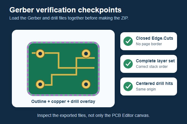
How to export Gerber files from KiCad, Gerber outline copper layers and drill hits checked together before manufacturing

Load the complete export: Open all Gerber layers, then load every Excellon drill file. The correct result is one entry for every expected copper, mask, silkscreen, profile, and drill output, with no file from an older revision.
Check the board outline: Edge.Cuts should show one continuous external profile plus only the intended internal cutouts. The displayed dimensions should match the source design, without a page border or unexpected outer rectangle.
Inspect copper in stack order: Toggle each copper layer and check that its routing, pads, planes, and board position belong to that layer. A multilayer set should contain every intended copper layer once, in the expected order.
Compare mask with pads: Solder-mask openings should align with exposed pads, test points, and other intended copper. Unexpected solid mask over a pad is a reason to return to the source board.
Review silkscreen clearance: Text should remain readable, appear on the intended side, and stay off exposed pads. In the finished-board view, bottom-side text should have the expected orientation rather than looking accidentally mirrored.
Overlay drill hits: Plated holes should sit inside their pads, while non-plated mounting holes and slots should align with the outline and mechanical features. A consistent offset across the board points to mismatched origins.
Check high-risk details: Zoom into fine-pitch footprints, connector rows, mounting holes, slots, board-edge features, and dense via fields. The correct export should preserve the same clearances and feature positions you approved in the source board.

A successful Plot message proves that KiCad wrote files; it does not prove that you selected every required layer or that the output represents the intended revision. When anything looks wrong, repair the source board, delete the affected export set, regenerate Gerbers and drills together, and repeat the viewer inspection.

What Should a Complete KiCad PCB Manufacturing Package Include?

Gerber files describe layer images and board geometry, but they do not communicate every manufacturing requirement. A complete handoff combines the exact files you inspected with the construction details that a fabricator cannot safely infer from those images.

Verified Gerber set: Include the same complete layer set that you loaded and checked in GerbView, without files from another revision.
Machine-readable drill data: Include the Excellon PTH and NPTH output generated for that Gerber set. A drill map is useful for review but is not a production drill file.
Stackup and construction details: State the layer order, material, finished thickness, copper weight, and any blind, buried, laser-drilled, filled, or capped via requirements.
Fabrication notes: Specify surface finish, controlled impedance, critical tolerances, panelization, special routing, and other order-specific requirements.
Optional Gerber job file: Include the .gbrjob file when generated and accepted, but do not use it instead of the individual Gerber, drill, and fabrication files.

If the same project also includes assembly, the assembler may request a BOM, component placement file, assembly drawings, paste layers, programming data, and test instructions. Those are PCBA inputs and should not be confused with the bare-board Gerber and drill package.

How Should You Package and Send KiCad Gerber Files to a Manufacturer?

Create the ZIP from the exact folder you inspected, then keep that verified archive unchanged for upload. This simple rule prevents a late file replacement from breaking the relationship between the viewer check and the package that reaches the manufacturer.

Start from an empty revision folder: Remove or archive the previous output before plotting. Never mix a new copper layer with an old outline or drill file.
Generate Gerbers and drills in one session: Matching timestamps are not a substitute for revision control, but they make accidental carryover easier to spot.
Verify that exact set: Load the folder’s Gerbers and drills into GerbView. Do not inspect one folder and ZIP another.
Use a clear archive name: Include the project and revision, such as controller-rev-b-fab.zip, without spaces or ambiguous words such as final-final.
Attach the fabrication notes: State quantity, material, stackup, finished thickness, copper weight, surface finish, impedance requirements, tolerances, delivery location, and any special process requirement that is not unambiguously encoded in the image files.
Review the manufacturer’s preview: If the upload portal renders the ZIP, compare the outline, layer count, dimensions, and drill pattern with your verified GerbView result before placing the order.

A .kicad_pcb file can be useful for engineering discussion, but it is not a universal substitute for fabrication output. Send it only when the manufacturer accepts native KiCad data and you are comfortable sharing the editable design. Keep the approved Gerber and drill archive as the order’s controlled manufacturing package.

Which KiCad Gerber Export Mistakes Cause Manufacturing Problems?

The most consequential errors are missing outline or drill data, wrong layer selection, mixed revisions, and inconsistent origins. The first symptom usually points to a narrow check, so correct the source or export decision instead of changing unrelated settings.

Issue	Impact and First Fix
Edge.Cuts missing or open	The board outline cannot be interpreted correctly. Close the outline and re-export Edge.Cuts.
Drill files omitted	Holes and vias are missing. Generate and include the Excellon drill files.
NPTH file omitted	Mounting or tooling holes may be missing. Include the separate NPTH drill file.
Inner layer missing	Multilayer connectivity may be incorrect. Check the stackup and re-export all copper layers.
Gerber and drill origins differ	Drill hits are shifted from pads. Use the same origin for both outputs.
Mixed revisions	Layers and holes may not align. Clear the output folder and export one revision.
Wrong extra layers included	The manufacturing package becomes ambiguous. Remove unrelated paste or fabrication outputs.
Files not inspected	Missing or shifted output may go unnoticed. Verify the exported files in GerbView.

Silkscreen over exposed pads is another frequent review finding, but it is not solved by selecting more files. Correct the source artwork or use the approved silkscreen-to-mask handling, then regenerate and inspect the affected silkscreen and mask layers.

FAQs About KiCad Gerber Export

Q1: Does the .gbrjob file include the drill data?

A1: No, the .gbrjob file does not include drill data. KiCad creates it as part of the Gerber export, while hole data is generated separately. Include the Excellon .drl files even when a .gbrjob file is present.

Q2: Can a drill map replace the .drl file?

A2: A drill map cannot replace the .drl file. It is a visual aid for reviewing hole locations and tool sizes. The manufacturer still needs the machine-readable drill file, normally in Excellon format.

Q3: How should slots and internal cutouts be included?

A3: Put board cutouts on Edge.Cuts and configure slots through their pad or drill properties. Use closed shapes for cutouts and set the correct plating property for each slot. Open the Gerbers and drill files together to confirm that every routed feature is present and aligned, and follow the manufacturer’s minimum slot and routing rules.

Q4: Why does the manufacturer’s preview show a full sheet or an oversized board?

A4: A page border or stray item is probably expanding the preview. Check that Plot drawing sheet is off, Edge.Cuts contains one valid closed outer profile, and Edge.Cuts was not added to every layer through Plot on all layers. The preview should show the board outline, not a full page or an unexpected rectangle.

Q5: Can KiCad open or edit the Gerber files after export?

A5: Use GerbView to inspect Gerbers, not as a substitute for the KiCad source design. GerbView can export limited geometry to PCB Editor, but that conversion does not recreate the original netlist, footprints, constraints, or full design intent. Make changes in the .kicad_pcb source, then export a new manufacturing set.

Q6: Do Gerber files include the BOM and component placement data?

A6: Gerber files do not include the BOM or component placement data. They describe the board’s fabricated layer images. Automated assembly normally requires a BOM and a component placement or centroid file in addition to the PCB manufacturing package.

Q7: Should I use different KiCad settings for JLCPCB or another manufacturer?

A7: Follow the manufacturer’s current requirements when they differ from KiCad’s general defaults. The essential checks stay the same: export every required layer, generate the drill files separately, keep the origins consistent, and inspect the exact upload package. A board-house profile does not replace GerbView inspection or the portal preview.

A reliable KiCad handoff comes from four controls: a checked source board, a complete layer and drill export, a viewer inspection of the actual files, and separate notes for requirements that images cannot fully express. That sequence is more dependable than copying a settings screenshot from a different KiCad release or manufacturer.

Once your KiCad Gerber and drill files have been verified, send the ZIP together with your stackup, material, copper weight, surface finish, impedance requirements, quantity, and delivery requirements to sales@bestpcbs.com. EBest Circuit can review the manufacturing package before PCB fabrication and provide a quotation based on the actual board requirements.

Star Grounding in PCB Design: When to Use or Avoid It

September 21st, 2026

Star grounding is a targeted fix for shared-return noise, not a default PCB layout style. It helps when a known high-current or noisy load would otherwise share return copper with a sensitive circuit, and the two branches can meet at one short, controlled junction. Fast digital, RF, and widely distributed currents usually need a continuous ground plane instead.

A sound choice starts with the actual current loops: identify the disturbing current, the reference that must stay quiet, the fastest edge, and every path that can reconnect the grounds. Those four facts lead to a practical decision between a star, a plane, or a hybrid layout and define what must be measured on the prototype.

Star grounding topology with four PCB return branches meeting at one controlled point

What Is Star Grounding, and What Problem Does It Solve?

Star grounding gives selected circuits separate return branches that meet at one controlled junction. The aim is to stop current from one branch flowing through the reference used by another branch before both currents reach their common source.

The problem is common-impedance coupling. Copper, vias, connectors, and solder joints all have impedance. When two circuits share a return segment, the current from the first circuit creates a voltage across that segment:

Reference error = shared return current × shared-path impedance

Consider a 24 V control board with a solenoid and a sensor amplifier. If the solenoid and amplifier share return copper, each solenoid current step can shift the amplifier reference and appear as a false sensor signal. Separate branches can keep the solenoid current out of the measurement path until both returns reach the supply reference.

The topology is useful only when the designer can name both sides of that relationship: the current that causes the error and the reference it disturbs. A radial drawing without that explanation is not a design decision.

How Do Frequency and Return Paths Affect Star Grounding?

Low-frequency load currents may tolerate separate branches, while fast-edge currents need a short return close to the outgoing signal. This is why a star can reduce sensor-reference error yet make a clock, data bus, or switching node worse.

Nominal operating frequency is not enough. A slowly updated bus may still switch in nanoseconds, and a low-sample-rate converter may contain fast clocks. Long branches add inductance and loop area, which can increase ringing, crosstalk, emissions, and susceptibility even when their DC resistance looks acceptable.

Check three things for every important signal or load:

The complete loop: source, outgoing conductor, load, and return conductor.
The fastest transition: driver rise and fall time, switch-node edge, converter clock, or ESD event.
Return continuity: plane splits, narrow necks, missing return vias, and connector boundaries that force a detour.

If a proposed branch sends a fast return across the board before it can close, use a nearby plane for that loop. The same PCB can still use a dedicated branch for a compact low-frequency load return.

When Does Star Grounding Work Well?

Star grounding works well when one identifiable load threatens one identifiable reference and both branches can reach a compact junction. The following conditions should all be true:

The disturbing current is known. Typical sources include a relay, motor, solenoid, heater, lamp, or power-output stage.
The sensitive reference is known. It may belong to a sensor, precision reference, measurement shunt, low-level audio input, or feedback network.
The junction is physically close. A supply return, bulk-capacitor return, regulator return, or connector boundary can accept the branches without long radial routing.
Fast local loops stay local. Decoupling, clocks, interfaces, and switching loops still close through a nearby plane or tightly coupled conductor pair.

On the control-board example, the solenoid can return directly to the power-entry capacitor while the sensor branch reaches the same reference on separate copper. The ADC and microcontroller interface can remain over continuous ground. This is a hybrid solution driven by current paths, not by the labels “analog” and “digital.”

When Should You Avoid Star Grounding and Use a Ground Plane Instead?

Avoid a whole-board star when fast signals, RF energy, dense routing, or distributed loads need many short return paths. Start with a continuous ground plane for most multilayer digital boards, then add a controlled junction only where a specific noisy branch must be kept out of a sensitive region.

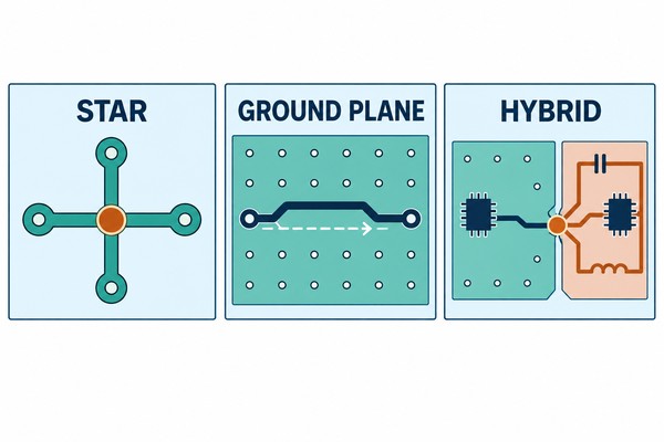
Engineering comparison of star, continuous ground plane, and hybrid PCB return topologies

Board condition	Starting topology	What to verify
One compact low-frequency load beside a sensitive reference	Star or Kelvin return	Measure reference movement during the worst load step.
Clocks, fast buses, RF traces, or rapid converter interfaces	Continuous ground plane	Keep an adjacent return path beneath the complete signal route.
Fast local interfaces beside a noisy power section	Hybrid	Keep fast returns on the plane and control where the power return joins it.
Loads spread across a large board	Plane or region-based power return	Calculate voltage differences using the actual routing length and current.
Several boards, cables, shields, or conductive mounts	System-level grounding plan	Trace every connection that can create a parallel return path.

A layout should be judged by return-current behavior rather than visual symmetry. A neat radial pattern can create a large high-frequency loop, while careful placement over a solid plane can keep a noisy load current away from a measurement circuit.

Where Should the Star Ground Point Be Placed?

Place the star point where the selected branch currents return to their shared source without crossing another branch’s reference first. That point is often near a bulk capacitor, regulator return, supply connector, or measurement shunt, not at the geometric center of the PCB.

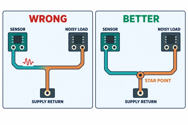
Engineering comparison of incorrect shared return routing and a controlled star point near the supply return

Mark the sources and loads. Include connectors, regulators, bulk capacitors, switching stages, sensors, converters, and external cables.
Draw outgoing and return current together. Check steady load, the worst load step, and the fastest transition because the paths may differ.
Locate the protected reference. Identify the exact point where the sensor, amplifier, ADC reference, or feedback network measures voltage.
Join the branches after their local reference points. The noisy current should reach the shared source without using the sensitive branch’s copper.

A net tie or zero-ohm resistor can make the chosen junction visible in the schematic and testable on the board. It cannot correct long branches or poor placement. Choose the electrical location first, then use the component or copper feature to enforce it.

How Should Analog, Digital, Power, and Chassis Grounds Meet?

Connect ground regions according to the currents they carry and the reference required by signals that cross between them. The names AGND, DGND, PGND, and chassis ground describe roles; they do not automatically require separate copper planes.

Analog return: keep load and switching current away from low-level inputs, references, and feedback nodes.
Digital return: give clocks and interfaces a short path beside their signal traces, even when average current is small.
Power return: contain converter hot loops, motor current, and gate-drive current near their sources and local capacitors.
Chassis, shield, and protective earth: route ESD, common-mode, shield, and safety current at the connector or enclosure boundary without sending it through a sensitive reference.

For a mixed-signal IC, follow the device data sheet and reference layout before splitting ground. AGND and DGND pins may describe internal circuit functions rather than a requirement for two board planes. The relevant questions are where the pin currents flow and what reference the crossing signals use.

Also trace paths outside the PCB. A cable shield, metal standoff, programming lead, or oscilloscope earth connection can bypass the intended junction. A board-level star is valid only if the assembled system preserves it.

What Layout Mistakes Make Star Grounding Fail?

Star grounding fails when the copper, components, or external connections create a different current path from the one shown on the schematic. These mistakes are the first places to look when the expected noise reduction does not appear:

The junction is beyond the sensitive reference. The noisy current crosses the measurement reference before reaching the star. Move the junction or change placement.
The branches are too long. A branch with acceptable DC resistance can still have excessive inductance. Keep fast returns on a plane.
A signal crosses a split or narrow ground neck. The return detours around the gap. Reroute the signal or restore continuous ground beneath it.
A second connection bypasses the star. Noise changes when a cable, enclosure, debugger, or instrument is attached. Trace current through the complete test setup.
Decoupling current travels to a remote junction. The IC supply loop becomes larger than necessary. Close each high-frequency decoupling loop locally.
A bead or zero-ohm link replaces analysis. The fitted part adds impedance but does not define the current path. Select it only after the target current and allowed voltage difference are known.

Change one path at a time during troubleshooting. Switch the suspected load while monitoring the protected reference, then repeat with the enclosure and external cables connected. The difference separates shared-copper error from a secondary path or radiated-coupling problem.

How Can You Review and Test a Star Ground Design?

A star-ground design is ready when the current-path drawing, physical junction, and measured result agree with one defined acceptance limit. Six checks provide that evidence:

Draw the critical loops. Mark the source, outgoing path, load, return, and local decoupling loop for each noisy, fast, or sensitive circuit.
Name the coupling. Record the aggressor current, shared path, victim reference, operating condition, and maximum acceptable error.
Compare the drawing with the PCB. Check branch length, plane continuity, layer changes, connectors, shields, mounts, and the exact junction feature.
Estimate the low-frequency error. Calculate shared resistance and voltage drop at maximum load and compare the result with the allowed reference shift.
Measure the load event. Compare idle and worst-load conditions with a short-ground-spring probe or an appropriate differential probe. Save the waveform that occurs at the same time as the disturbing event.
Repeat the test on the assembled system. Add the enclosure, shields, cables, debugger, and representative external equipment so hidden return paths are included.

The result should lead to one decision. Keep the star if the protected reference stays within its limit and fast local returns remain continuous. Use a plane or hybrid if fast or distributed currents need a nearby reference. Change the architecture if the current paths or acceptance limit are still unclear.

FAQs About Star Grounding

Q1: Should each star-ground branch use a separate schematic net name?

A1: Use separate net names when they help the CAD tools enforce the intended connection. Join them with a documented net tie or approved junction footprint, then confirm that the PCB netlist and copper contain no unintended second connection.

Q2: How wide should a star-ground branch be?

A2: Size it from current, allowable voltage drop, temperature rise, and transient behavior. There is no universal width. A high-current branch may need wide copper, while a sensing branch may need a separate Kelvin path that carries almost no load current.

Q3: Can a ground pour surround star-ground branches?

A3: Yes, but the pour must not create a parallel connection between branches. Use clearances or a controlled net-tie strategy, then inspect the final Gerber data and connectivity report rather than relying on the schematic alone.

Q4: Can several regulators share one star point?

A4: They can when their return currents meet at a low-impedance source node without modulating another regulator’s reference. If one converter has large switching or load-step current, give it a local hot loop and check whether a higher-level junction is needed.

Q5: How should star-ground noise be measured with an oscilloscope?

A5: Measure between the protected reference and its source reference during the suspected load event. Use a short ground spring or a suitable differential probe; a long probe ground lead can create a loop and show noise that is not present at the circuit node.

Conclusion: Choose the Grounding Topology from the Current Loops

Choose a star only for a specific shared-impedance problem that has short branches, a clear victim reference, and one practical convergence point. Choose a continuous plane when fast or distributed currents need nearby returns. Use a hybrid when those two needs exist on the same board.

The next design review should produce two items: an annotated drawing of the critical current loops and a measurement plan for the worst load event. If both are specific, the topology choice can be checked. If either remains vague, deciding between star grounding and a ground plane is premature.

What Is the Relative Permittivity of FR4? Typical Dk Values and PCB Design Considerations

September 15th, 2026

The relative permittivity of FR4 is commonly estimated at about 4.4. That estimate is useful during early layout, but the final Dk depends on the laminate system, glass-resin construction, frequency, test method, and modeling purpose. These distinctions affect controlled-impedance geometry, effective signal velocity, propagation delay, and phase, so a reliable PCB design separates reference Dk, measured datasheet Dk, Design Dk, and effective permittivity before trace geometry or timing limits are finalized.

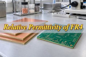
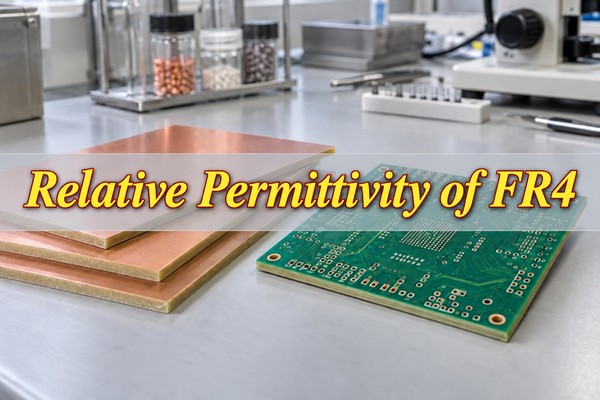
Relative Permittivity of FR4, titled hero with copper-clad laminate sheets and a fabricated PCB

What Does Relative Permittivity Mean in FR4?

Relative permittivity of FR4, written as εr and commonly called dielectric constant or Dk, is the ratio between the material’s permittivity and the permittivity of a vacuum. Because it is a ratio, Dk has no unit. A material with a higher Dk stores more electric-field energy than a material with a lower Dk under the same field conditions.

On a PCB, that stored field energy contributes to the capacitance per unit length of a trace. Capacitance and inductance together set the trace’s characteristic impedance and propagation velocity, which is why Dk appears in transmission-line and stackup calculations. Dk should not be confused with dissipation factor, or Df: Dk primarily influences impedance and phase velocity, while Df describes dielectric energy loss.

The laminate Dk is also different from the effective permittivity experienced by a finished trace. A microstrip shares its electric field between the laminate and air, while a stripline contains almost all of its field within dielectric. The same laminate can therefore produce different effective signal velocities on different layers.

What Is the Typical Relative Permittivity of FR4?

About 4.4 is the usual general-reference value for FR4. A preliminary range of approximately 4.0–4.4 is reasonable when the material and stackup have not yet been chosen, but neither value is precise enough to release controlled-impedance geometry. Once a laminate construction is selected, the model should use data that matches that construction, the intended frequency range, and the type of calculation.

Design Stage	Dk Input
General reference	About 4.4
Early estimate	About 4.0–4.4
Selected laminate	Construction-specific data
Controlled impedance	Applicable Design Dk
Broadband or RF model	Frequency-dependent data

These values belong to different levels of design certainty. The preliminary range can reserve routing space and expose an obviously impractical stackup. It cannot confirm final trace width because the actual glass style, pressed dielectric thickness, copper geometry, and modeling Dk remain unknown. The Dk input should become more specific as the electrical requirement becomes less tolerant of variation.

How Do Glass Weave and Resin Content Affect FR4 Permittivity?

FR4 is a composite of glass reinforcement and cured resin, and the two constituents have different permittivity. Glass-rich constructions generally produce a higher composite Dk, while resin-rich constructions generally produce a lower value. Glass style also changes the distribution of resin and glass through the dielectric, so two cores from the same laminate family can require different Dk inputs.

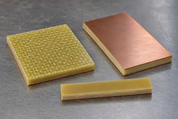
Relative Permittivity of FR4, glass weave, resin laminate, and copper-clad samples

The table compares published typical core data for two FR408HR constructions measured under the same reported frequency points.

Construction	Resin	100 MHz	1 GHz	10 GHz
106	72%	3.37	3.34	3.30
1080	57%	3.67	3.62	3.59

At 1 GHz, the 1080 core is reported at 3.62 and the more resin-rich 106 core at 3.34, a difference of 0.28. That is about 8.4% relative to the 106 value and is large enough to change a controlled-impedance solution. These are typical core values for the stated constructions, not interchangeable values for every core or prepreg. Final impedance and delay models should identify both the laminate grade and the production construction.

Glass weave also creates small local changes in field environment. A narrow trace may run mainly over a resin-rich opening or closer to glass bundles, which can contribute to pair-to-pair skew in demanding high-speed designs. Routing angle, wider traces, spread-glass options, and tighter construction control can reduce that sensitivity when the available timing margin makes it relevant.

How Does Frequency Affect the Relative Permittivity of FR4?

FR4 is dispersive, so its reported Dk changes with frequency. In the FR408HR 106-core example, the published value is 3.37 at 100 MHz, 3.34 at 1 GHz, and 3.30 at 10 GHz. The decrease from 100 MHz to 10 GHz is approximately 2.1%.

A small percentage change can still matter over a long route or a narrow phase budget. It changes effective permittivity, shifts calculated impedance, and accumulates as propagation delay. A solver that accepts one Dk value should therefore use a value near the band that drives the electrical requirement. A broadband model may require a dispersive material model rather than one fixed point.

For digital channels, clock frequency is not the only frequency reference. Edge rate determines how much high-frequency spectral energy the interconnect must carry, while channel bandwidth and loss determine which part reaches the receiver. A low clock rate with fast edges can require material data at frequencies well above the clock fundamental. Rise time, channel bandwidth, and the required phase or delay accuracy provide a better basis for selecting the relevant Dk data.

How Do Test Methods Affect Reported FR4 Dk?

A Dk result is meaningful only with its test method, frequency, and specimen condition. Parallel-plate, clamped-stripline, resonator, and circuit-based methods create different field distributions and handle fixture and specimen effects differently. Values produced by different methods can therefore disagree even when both measurements are valid.

Specimen thickness, resin content, copper removal, surface condition, clamping pressure, and air gaps can influence the result. Material anisotropy adds another distinction: an in-plane transmission-line measurement does not necessarily represent the same dielectric direction as a through-thickness capacitance method. Comparing two numbers without these conditions can create a false material difference.

When two sources report different Dk values, compare the method, test frequency, construction, sample conditioning, and whether the value is a measured specification or a design recommendation. Values should be transferred into the same model only when those conditions and intended uses are compatible.

What Is the Difference Between Datasheet Dk, Design Dk, and Effective Permittivity?

Datasheet Dk describes a published material result, Design Dk is intended for transmission-line modeling, and effective permittivity belongs to a specific trace structure. Treating the three as synonyms is a common source of impedance and delay errors.

Datasheet Dk: A value reported for a stated material, specimen, frequency, and test method. It supports material comparison only when the reported conditions are comparable.
Design Dk: A laminate value selected or derived to improve correlation between transmission-line calculations and fabricated circuits. It is the preferred material input when the supplier provides it for the relevant product, construction, and frequency.
Effective permittivity, εeff: The field-weighted value experienced by a particular microstrip, stripline, or coplanar structure. Geometry, layer location, solder mask, and the surrounding media all influence it.

For a microstrip, part of the field travels through air, so εeff is normally below the laminate’s bulk or Design Dk. A stripline is surrounded by dielectric and its εeff is usually closer to the laminate value. An effective microstrip value is not a valid laminate input when the field solver expects bulk or Design Dk. The material value goes into the model; the solver then calculates the structure’s effective behavior.

How Does FR4 Permittivity Affect PCB Impedance?

With geometry held constant, a higher Dk generally lowers characteristic impedance. Transmission-line impedance is related to the ratio of inductance to capacitance per unit length. A higher material permittivity increases electric-field storage and capacitance, reducing impedance unless the geometry changes.

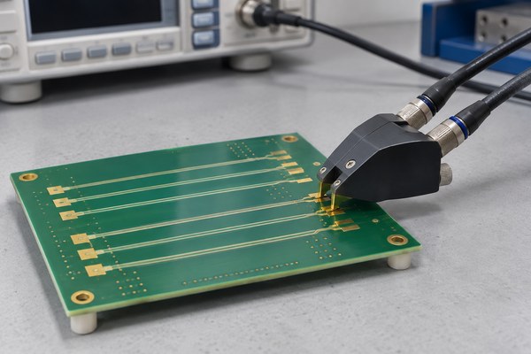
Relative Permittivity of FR4, controlled-impedance coupon and differential probe

For a 50 Ω single-ended line, a Dk increase may require a narrower trace or greater distance to the reference plane. Differential impedance also responds to pair spacing because coupling changes the even- and odd-mode capacitance. Copper thickness, trapezoidal etch shape, solder mask, and finished dielectric thickness modify the result at the same time, so a Dk percentage change does not translate into an equal percentage change in impedance.

The practical check is a sensitivity run using the proposed production stackup. Calculate the nominal line, then repeat the model at the expected Dk and geometry limits. If the resulting impedance range exceeds the drawing tolerance, the design needs a different geometry, a tighter construction, or a more controlled laminate definition before routing is frozen.

How Does FR4 Permittivity Affect Signal Speed and Propagation Delay?

A higher effective permittivity reduces wave velocity and increases propagation delay. For a simplified nondispersive transmission line, v ≈ c / √εeff. The corresponding delay is approximately 84.7 ps/in × √εeff.

At εeff = 3.2, the estimated delay is about 151.5 ps/in. At εeff = 3.6, it is about 160.8 ps/in. Across a 10-inch route, the difference is approximately 93 ps. This comparison isolates the effect of εeff and is not a universal FR4 delay value.

Delay variation matters when it consumes setup-and-hold margin, pair skew, phase alignment, or a length-matching budget. Layer changes deserve particular attention: a microstrip and stripline can have different εeff even when they use the same laminate system. Matching copper length alone does not guarantee equal electrical delay when two routes see different constructions or field distributions.

For timing review, convert the modeled delay into ps/in for each relevant layer and compare the accumulated difference with the available budget. That check is more reliable than applying one generic propagation factor to every layer in the stackup.

Which FR4 Permittivity Value Should You Use for PCB Design?

The correct Dk input depends on the design stage and the decision being made. Early placement needs a plausible estimate; released impedance and timing constraints need construction-specific data.

Preliminary PCB design: Use about 4.0–4.4 as a documented assumption while the material remains open. Model more than one value if routing space is tight, and avoid fixing the final trace width from this estimate.
Selected laminate: Use data for the chosen product and glass-resin construction at the relevant frequency. Confirm whether the stated number is a test-method result or the supplier’s recommended modeling value.
Controlled-impedance or high-speed PCB: Use the applicable Design Dk with the finished dielectric thickness, copper geometry, solder-mask condition, and a construction that can be supported in production.

A value of 4.4 is useful for early feasibility work, but it should not automatically become the released Dk for a controlled-impedance board. Before final routing, the laminate identity, construction, frequency basis, solver definition, and proposed stackup should describe the same physical build.

When Is a Generic FR4 Dk Value No Longer Accurate Enough?

A generic value stops being adequate when Dk uncertainty consumes a meaningful share of the electrical margin. The decision is set by the channel requirement, not by one universal frequency threshold.

Impedance margin is narrow: Model the expected Dk and geometry limits. If the calculated range approaches or exceeds the impedance tolerance, use controlled construction data and agree on achievable finished dimensions.
Delay, skew, or phase is tightly budgeted: Convert Dk uncertainty into delay across the actual route length and layer transitions. Construction-specific data is needed when that uncertainty is no longer small relative to the timing budget.
The channel is broadband or loss-sensitive: Review Dk dispersion and Df over the band that reaches the receiver. A single low-frequency value cannot describe broadband phase and loss behavior.
A laminate substitution is proposed: Compare construction, Design Dk, Df, and finished dielectric thickness, then recalculate impedance and delay. Matching Tg or nominal board thickness does not establish electrical equivalence.

When the modeled worst case leaves insufficient margin, the practical choices are tighter construction control, a laminate with better-characterized electrical data, a revised stackup, or more tolerant routing constraints. This connects material selection directly to the requirement that is at risk.

FAQs About FR4 Relative Permittivity

Q1: Is the relative permittivity of FR4 always 4.4?

A1: No. About 4.4 is a general estimate; actual values vary with laminate formulation, glass-resin construction, frequency, and test method.

Q2: Is relative permittivity the same as dielectric constant?

A2: Yes in PCB material discussions. Relative permittivity, dielectric constant, εr, and Dk commonly identify the same material property.

Q3: Does FR4 Dk change with frequency?

A3: Yes. FR4 is dispersive, so the modeling value should correspond to the relevant signal band.

Q4: Does PCB thickness affect FR4 permittivity?

A4: Board thickness does not directly redefine Dk, but achieving a different thickness can require another glass-resin construction with different electrical data.

Q5: What FR4 Dk should be used for a 50-ohm trace?

A5: Use the applicable Design Dk for the selected construction and solve it with the finished trace and stackup geometry.

Q6: Is effective permittivity the same as FR4 Dk?

A6: No. FR4 Dk is a laminate property; effective permittivity is the field-weighted result for a particular transmission-line structure.

Q7: Why do different FR4 datasheets show different Dk values?

A7: The products, constructions, frequencies, specimen conditions, test methods, or reporting purposes may differ.

Q8: Does FR4 permittivity affect signal propagation speed?

A8: Yes. Higher effective permittivity generally reduces wave velocity and increases propagation delay.

FR4 has no single Dk that fits every PCB calculation. About 4.4 is suitable for early estimates, while controlled-impedance, timing-sensitive, and broadband designs need a value tied to the selected laminate, glass-resin construction, relevant frequency, and modeling method. That distinction keeps the material data, stackup geometry, impedance target, and delay calculation consistent.

If your PCB requires controlled impedance, high-speed routing, or a tight delay budget, send the layer count, target impedance, preferred laminate if known, and key interface to sales@bestpcbs.com. BestPCBS can review the proposed stackup and Dk assumptions before the trace geometry is finalized.

Difference Between Offshore and Domestic PCB Manufacturers

September 15th, 2026

The difference between offshore and domestic PCB manufacturers is the location of the factory that performs the released fabrication or assembly work. That location affects total delivered cost, receiving lead time, available processes and capacity, engineering access, quality oversight, and recovery after a delayed or rejected lot. Neither route is automatically cheaper, faster, or better.

OEMs, EMS providers, and product teams need more than a country label. They need to know which factory will build the boards, what the complete delivered cost will be, when usable boards will arrive, and how a failed lot will be recovered. Those answers make it possible to match the sourcing route to the design stage, volume, deadline, and business risk.

difference between offshore and domestic PCB manufacturers, finished printed circuit boards on a professional inspection bench

What Is the Difference Between Offshore and Domestic PCB Manufacturers?

The difference between offshore and domestic PCB manufacturers is the factory location—not the sales address. Domestic manufacturing keeps the quoted fabrication or assembly in the buyer’s home country. Offshore manufacturing assigns that work to a factory abroad. This distinction applies only to the production location; a domestic legal supplier may still use an offshore factory.

Criteria	Domestic Manufacturing	Offshore Manufacturing
Manufacturing Site	Factory in the buyer’s home country	Factory outside the buyer’s home country
Order Profile	Prototypes, NPI, frequent ECOs, and urgent replenishment	Released designs, repeat volume, and planned releases
Cost Structure	Higher conversion cost may be offset by lower freight, duty, and buffer-inventory exposure	Lower conversion cost may be available at scale; freight, duty, and inventory remain part of delivered cost
Lead Time	Shorter transit and recovery cycle	Longer transit and customs path; better suited to planned releases
Engineering Interface	More working-hour overlap and easier site access	Scheduled cross-time-zone reviews and stronger written control
Supply-Chain Risk	Smaller qualified pool or constrained local capacity	Freight, customs, currency, and regional disruption

How Do Offshore and Domestic PCB Manufacturing Costs Compare?

Offshore production can reduce the factory price on repeat orders, while domestic production can reduce freight, import charges, buffer stock, and urgent-recovery expense. Compare total landed cost per accepted board—not the quoted unit price.

Calculate both quotations on the same basis:

Total landed cost per accepted board = production price + tooling/NRE + freight + insurance + duty and brokerage + payment or currency cost + incoming inspection + expected scrap or rework + inventory carrying cost + recovery cost, divided by accepted quantity.

The result usually turns on three project conditions:

Small or changing orders: Tooling, first-article review, engineering exchanges, expedited freight, and another revision can outweigh a modest unit-price saving.
Stable repeat demand: Panel utilization, quantity breaks, planned material purchasing, scheduled freight, and controlled buffer stock can strengthen the offshore cost case.
Expensive nonconformance: Sorting, rework, replacement production, return freight, and lost line time can erase an apparent saving from either route.

Put both offers on the same shipment size, freight mode, delivery term, importer responsibility, inspection scope, and recovery assumption. Only then can the buyer see whether an offshore factory-price advantage remains at the receiving dock.

How Does Lead Time Differ Between Domestic and Offshore PCB Manufacturers?

Domestic production usually reaches the buyer sooner for prototypes and emergency replacements. Offshore production can still meet a planned schedule when materials, capacity, approvals, and air freight are secured in advance. Measure lead time from the release of complete data to the receipt of usable boards.

For a U.S. buyer, the ranges below are practical RFQ estimates when the data package is complete, common materials are available, no major engineering hold occurs, and offshore shipments travel by express or air freight.

Order Type	Domestic Lead Time	Offshore Lead Time	Main Variables
Simple prototype bare boards	3–10 business days	7–15 business days	Layer count, quick-turn capacity, DFM questions, material availability, and courier pickup
Standard multilayer, low-volume order	10–20 business days	15–30 business days	Lamination cycles, via filling, controlled impedance, surface finish, test records, and customs
Repeat production order	3–5 weeks	4–7 weeks by air	Forecast release, panel utilization, material allocation, production queue, inspection, and freight booking
PCB assembly after all parts are ready	About 2–4 weeks	About 3–5 weeks	Stencil preparation, placement complexity, BGA or bottom-terminated components, test scope, rework, and shipment release

A committed delivery date must include material readiness, factory capacity, inspection, freight, customs, and final delivery. Domestic production has the clearer advantage when rapid recovery matters; a prepared offshore source can remain competitive for scheduled orders.

How Do Manufacturing Capabilities Compare Between Offshore and Domestic PCB Manufacturers?

Domestic factories often handle prototype feedback and engineering changes more quickly. Offshore factories may provide greater production scale or a broader integrated supply network. Neither location proves technical capability; the assigned factory must demonstrate that it can build the released design.

Capability	Domestic	Offshore	Verification
Prototype and NPI	Often supports shorter DFM and revision loops for small builds	Works best with stable data and controlled approval windows	DFM response, prototype equipment, revision cutoff, and sample schedule
Advanced fabrication	Available through qualified specialist factories	Available through qualified factories and, in some cases, a wider production network	Exact site, process route, equipment, feature limits, and in-house or subcontracted scope
Materials	Local stock can shorten replenishment; specialist laminates may still be imported	Regional supply networks may broaden options but still face allocation and transit risk	Approved material, manufacturer, grade, stock status, alternate rules, and replenishment lead time
PCB assembly	Useful when hands-on debug, low-volume changes, or local validation is important	Can combine sourcing, assembly, inspection, and volume production in one route	Placement range, BGA capability, X-ray, programming, test scope, and rework control
Production volume	May suit low-volume or specialist work; available capacity must be confirmed	Can offer stronger panel utilization and repeat-volume capacity when reserved	Monthly capacity, bottleneck equipment, material allocation, ramp plan, and queue position
Backup production	Physical oversight can be easier, but the qualified local pool may be smaller	Additional sites may be available, although transfer control becomes more complex	Matched stackup, tooling, approved materials, test method, change control, and transfer validation

Choose the route that fits the design stage and order scale, then qualify the factory against the released stackup, materials, vias, tolerances, assembly, testing, and capacity requirements. The factory record—not its country—establishes capability.

Does PCB Quality Differ Between Domestic and Offshore Manufacturers?

Neither geography has a built-in quality advantage. A domestic or offshore board is only as reliable as the factory’s control of materials, drilling, plating, imaging, inspection, testing, and corrective action. Use the same acceptance criteria for both routes, then compare the records from the actual production lot.

PCB quality inspection for domestic and offshore manufacturing comparison

Look for the following controls before approving either source:

Material and stackup control: The released material, copper, finished thickness, stackup, surface finish, tolerances, and approved substitutions match the production records.
Drilling and plating control: Hole preparation, plating, filled-via processes, registration, and microsection evidence address the features that carry the greatest reliability risk.
Inspection and test plan: Electrical test, impedance data, coupons, automated or visual inspection, X-ray where applicable, sample size, limits, units, and report format are agreed before production.
Certificate scope: Any required certificate identifies the correct legal entity, manufacturing site, covered activity, and valid period.
Lot traceability: Material lots, work orders, approved deviations, inspection records, and shipment records remain connected to the delivered lot.
Change control: Site, material, stackup, finish, subcontractor, and controlled test-method changes require approval before use.
Corrective action: Containment, root-cause analysis, replacement, effectiveness checks, and recurrence prevention have named owners and defined outputs.

Domestic sourcing can make an on-site audit or urgent physical review easier. An offshore source can deliver the same level of control when the order defines the required records, samples, approvals, and escalation path. Give preference to the factory that can trace how the lot was built, tested, released, and corrected when a result falls outside the agreed limit.

How Do Communication and Engineering Support Differ?

Domestic manufacturing generally offers more overlapping work hours and easier site access. Offshore manufacturing relies more heavily on complete written records and scheduled approval windows. What matters is whether questions reach the right engineer, decisions are recorded, and production waits for required approval.

Test that process with real project questions before placing the order:

Named technical owner: Identify who receives DFM questions, who can answer process questions, and who owns escalation when the normal contact is unavailable.
Written DFM record: Require stackup, impedance, material substitution, drill or via, panelization, assembly, and test questions to remain tied to the correct data revision.
Approval authority: Record which changes require engineering approval and which manufacturing adjustments are already permitted by the released notes.
Revision control: Use one controlled package for Gerber or ODB++, drill data, drawings, BOM, placement data, and approved responses so that fabrication and assembly do not work from different versions.
Response expectations: Agree how urgent questions are flagged, when overlapping working hours are available, and how an unanswered issue affects the production schedule.
ECO handoff: Confirm how an engineering change closes open work, identifies affected inventory, and authorizes the next build revision.

A domestic source may resolve an urgent question during the buyer’s working day and arrange a visit more easily. An offshore source can keep the project moving when ownership, revision history, approval authority, and escalation timing are explicit. Judge the communication process by how clearly questions are closed, not by time zone alone.

What Supply Chain and Logistics Risks Should You Compare?

Domestic and offshore routes fail in different ways. A domestic route may depend on a smaller qualified supplier pool or limited special-process capacity; an offshore route adds freight, customs, currency, and a longer replacement path. The better route is the one whose likely disruption the program can absorb and recover from.

PCB production shipment prepared for offshore supply chain and logistics

Domestic continuity checks should cover:

Qualified capacity: Confirm material allocation, critical equipment, queue position, and the plan for an unexpected increase in demand.
Special-process availability: Identify which required constructions, finishes, materials, and tests depend on a single local site or subcontractor.
Single-source exposure: Determine whether another domestic or offshore factory could reproduce the released build without an uncontrolled transfer.
Cost concentration: Review price breaks and capacity reservations across the forecast rather than treating a prototype quotation as production economics.

Offshore continuity checks should cover:

Freight route: Set the shipment mode, handoff points, carrier buffer, insurance, and contingency for a missed booking or transport disruption.
Customs responsibility: State the importer of record, classification owner, documentation, duty basis, brokerage, and delivery term in the quotation.
Commercial exposure: State the quotation currency, validity, payment timing, and treatment of material commitments if demand changes.
Regional concentration: Identify whether the factory, material source, port, and backup route depend on the same geographic event.
Replacement route: Agree how a delayed or rejected lot will be contained, sorted, remade, and shipped without waiting for an undefined return process.

Before awarding the order, model three events: a factory stoppage, a missed receiving date, and a lot rejected at incoming inspection. Choose the route that keeps downtime, cash exposure, and recovery time within the program’s limits.

When Is a Domestic PCB Manufacturer the Better Choice?

Choose a domestic PCB manufacturer when proximity materially shortens engineering, validation, audit, or recovery work. Domestic production is usually the better fit for changing designs, small urgent builds, location-restricted programs, and demand that cannot support long transit or inventory buffers.

Early prototypes: Engineers need quick feedback on stackup, tolerances, materials, assembly details, or test access before the design is frozen.
Frequent revisions: Several ECOs are expected, and the cost of obsolete work or material exceeds the expected unit-price saving.
Small urgent builds: Validation, repair, service, or replacement quantities must arrive quickly and cannot absorb a large minimum order.
Fast failure recovery: A rejected lot could stop a launch or production line, making nearby sorting, rework, or replacement capacity valuable.
Physical oversight: The buyer needs a short-notice audit, witness point, process review, or in-person corrective-action meeting.
Location restrictions: Contract, customer, data, end-use, or site-access requirements limit where the board may be fabricated or assembled.
Unstable demand: Release quantities and dates change often enough that excess inventory becomes a larger risk than unit price.

A domestic premium is justified when the shorter loop prevents a costly delay, obsolete revision, or compliance problem. The factory must still prove its process capability, capacity, quality records, and commercial terms; proximity alone is not a qualification.

When Is an Offshore PCB Manufacturer the Better Choice?

Choose an offshore PCB manufacturer when the design is stable, demand is forecastable, the proposed location is permitted, and the cost or capacity advantage remains after logistics and risk are included. Offshore production works best when materials, capacity, and shipments can be planned before the order becomes urgent.

Stable production data: Stackup, materials, fabrication notes, BOM, placement data, inspection criteria, and approved substitutions are controlled under one revision.
Repeat volume: Medium- or high-volume demand can benefit from panel utilization, material purchasing, scheduled production, and quantity pricing.
Broader process access: The proposed site can show a suitable route for HDI, rigid-flex, high-frequency materials, heavy copper, metal-core, ceramic, or coordinated PCBA requirements.
Predictable releases: Forecasts, material commitments, shipment windows, and inventory rules can absorb international transit.
Available production capacity: The offshore candidate can reserve the equipment, material, and queue position needed for the planned ramp.
Mature remote control: DFM approvals, revision control, lot records, nonconformance handling, and corrective action follow a documented process.
Permitted manufacturing route: Customer, contract, file-control, end-use, production-country, and shipment-destination rules allow the assigned site.

An offshore advantage is real only when it survives a complete receiving-date and landed-cost comparison and the factory can provide the required technical and quality records. If freight, buffer stock, or recovery exposure removes the saving, the unit price does not justify the route.

How Should You Choose Between Offshore and Domestic PCB Manufacturers?

Eliminate unsuitable routes before comparing price. Start with non-negotiable location and capability requirements, then compare lead time, landed cost, quality evidence, and recovery among the factories that remain.

Check manufacturing-location restrictions: Remove any fabrication or assembly site that conflicts with customer, contract, data, end-use, or site-access requirements.
Match the required technologies: Confirm that the assigned factory can control the actual stackup, materials, vias, tolerances, finishes, electrical requirements, assembly, and tests.
Assess design stability: Decide whether the next order is a changing prototype, a validation build, or released repeat production.
Set the receiving date: Work backward through engineering release, materials, production, verification, transit, customs, and incoming acceptance.
Use the real order profile: Compare the prototype quantity, production breaks, release pattern, ramp forecast, and likely material commitments.
Normalize landed cost: Put production, tooling, freight, import charges, inspection, inventory, scrap, rework, and recovery on the same delivery basis.
Set the release evidence: State the inspection reports, electrical or impedance results, traceability, certificates, deviations, and approvals needed for acceptance.
Model a disruption: Calculate what happens if production stops, a shipment is delayed, or a lot is rejected at receiving.
Compare recovery speed: Ask who contains the issue, what evidence arrives first, where replacement work is performed, and when conforming boards can be restored.
Choose the source structure: Use one source when its continuity plan covers the risk; qualify a second source when the transfer cost is justified and both routes can build the same released design.

Changing prototypes and urgent deliveries often favor domestic production; stable repeat orders with planned demand can favor offshore production. For a complex PCB, qualify the factory’s process capability before using geography as a deciding factor.

Why Choose EBest Circuit for Offshore PCB Manufacturing?

When offshore production suits the project, EBest Circuit can quote PCB fabrication, component sourcing, assembly, agreed testing, and delivery as one scope. Engineering, quality, and purchasing can review the same technical assumptions, responsibilities, and delivery basis before releasing the order.

Spend less time coordinating suppliers: One request can cover bare boards, components, assembly, testing, packaging, and delivery instead of requiring separate quotations.
Resolve technical issues earlier: DFM review can close stackup, material, via, panelization, assembly, and test questions before material is committed.
Match the factory to the design: HDI, rigid-flex, high-frequency, heavy-copper, metal-core, ceramic, volume, and assembly requirements can be screened before order placement.
Compare the complete cost: Quantity breaks, tooling, included services, packaging, delivery terms, and buyer responsibilities can be shown in one commercial scope.
Improve traceability and recovery: Revision status, inspection records, shipment milestones, escalation, and replacement expectations can be agreed before production begins.

This reduces supplier handoffs and makes the offshore quotation easier to compare with a domestic offer. Projects that require domestic manufacturing should remain with a qualified domestic source.

FAQs About Offshore and Domestic PCB Manufacturers

Q1: Is offshore PCB manufacturing the same as outsourcing?

A1: No. Outsourcing describes who performs the work; offshore describes where it is performed. A buyer can outsource fabrication or assembly to a domestic factory, an offshore factory, or separate factories in both locations. The distinction determines which location, trade, delivery, and recovery controls apply.

Q2: Is nearshore PCB manufacturing considered offshore?

A2: Yes, when the factory is outside the buyer’s home country. Nearshore production may reduce distance, time-zone difference, or freight exposure, but the manufacturing route is still cross-border. Price the border, transport, and recovery steps as a distinct route.

Q3: Are offshore PCB manufacturers always cheaper?

A3: No; the answer can change by order size and delivery method. Recalculate the comparison when quantity, freight mode, duty treatment, material commitment, inspection scope, or expected rework changes rather than carrying a savings percentage from one build to the next.

Q4: Are domestic PCB manufacturers always faster?

A4: No; factory capacity and material readiness can outweigh distance. Require both suppliers to state when the schedule starts, which customer approvals can stop it, and whether the quoted date is factory completion, shipment, or usable receipt.

Q5: Can offshore PCB manufacturers meet the same quality requirements as domestic suppliers?

A5: Yes, when the assigned site can meet the same specification and release evidence. Audit access may differ, so specify the lot records, test reports, traceability, deviation approval, and corrective-action outputs that must be available remotely.

Q6: Can bare PCBs be produced offshore and assembled domestically?

A6: Yes, but the two sites must be qualified separately. Set bare-board incoming inspection, packaging and moisture controls where applicable, ownership during transit, rejection handling, and the date accepted boards must reach the assembly line. Assign a named owner to every handoff.

Q7: How do Incoterms affect offshore PCB cost?

A7: They assign delivery tasks, cost, and risk between buyer and seller. Compare quotations at the same named place and version of the chosen term, then identify who books freight, carries insurance, clears customs, pays duties, and manages final delivery.

Q8: Should prototype and mass production use the same PCB supplier?

A8: Only when the supplier can control the transfer as well as both build stages. Compare prototype speed, volume equipment, panelization, approved materials, tooling, test coverage, revision history, and the evidence used to release the first production lot.

Q9: Can domestic and offshore PCB manufacturers be used as dual sources?

A9: Yes, if both sources build the same controlled product specification. Align stackup, approved materials, fabrication notes, test method, acceptance limits, revision control, and change approval; otherwise the backup may produce a materially different board when it is needed.

Q10: What documents should be requested from an offshore PCB manufacturer?

A10: Request the records that prove the assigned site, released construction, inspection result, and lot identity. Depending on the order, this may include site and process confirmation, stackup approval, material or conformity records, electrical and impedance results, microsection or inspection reports, approved deviations, packing details, and shipment traceability.

If you are comparing domestic and offshore options for an upcoming PCB build, send EBest Circuit your Gerber or ODB++ files, stackup, materials, quantity, destination, and required delivery date. For assembly, include the BOM and placement files. Email sales@bestpcbs.com, and we can prepare a project-specific PCB or PCBA quotation.

What Does IPC-6012 Class II Mean for Your PCB?

September 11th, 2026

IPC-6012 class II identifies a performance level for rigid printed circuit boards used in dedicated-service electronics. Usually written Class 2, it addresses the quality of the manufactured bare board, including its conductors, plated holes, insulation and structural integrity. It is not simply an appearance grade. At EBest Circuit (Best Technology), we manufacture PCBs and help you connect the specified performance class with a practical board construction, so your assembly starts with the right foundation.

Conceptual illustration of IPC-6012 Class II rigid PCB quality with a plated board and inspection coupon

What Is IPC-6012 Class II?

IPC-6012 Class II means the Class 2 requirements within the qualification and performance specification for rigid printed boards. Class 2 serves equipment where dependable operation and an extended service life matter, but uninterrupted operation is not as critical as it is for Class 3 applications. The numeral II does not mean a two-layer board or revision two of the standard.

IPC 6012 class 2 can apply to different rigid constructions, from a double-sided controller board to a multilayer interconnect. Layer count, laminate grade and surface finish still need their own specification. A Class 2 designation therefore answers one important question about acceptance, but does not define every feature of your PCB.

Which Products Are Suitable for Class 2 PCBs?

Class 2 is a relevant starting point for many commercial instruments, communications peripherals and industrial controls whose service requirements match dedicated-service electronics. The application name alone does not determine the class: the consequence of failure and the required operating conditions matter more.

Application example	What the PCB contributes	What still needs application-specific attention
Commercial measurement instrument	Stable connections between sensing, conversion and display circuits	Leakage paths, noise-sensitive layout and calibration requirements
Communications peripheral	Interconnects for processing, power and external interfaces	Controlled impedance, connector loading and signal integrity
Non-safety-critical industrial controller	Reliable mounting and connections for control and input/output circuits	Temperature cycling, contamination and terminal mechanical loads

Conceptual industrial controller assembly showing a rigid PCB application, not a customer product or conformity claim

For these types of circuits, our FR4 printed circuit boards provide a manufacturing route from prototypes to multilayer builds. We review the board design against the requested construction; an instrument’s safety function or environmental exposure may require additional requirements beyond a general Class 2 designation.

What Do IPC 6012 Class 2 Requirements Cover?

IPC 6012 class 2 requirements cover the finished bare board’s physical and electrical quality, not just its visible surface. The areas below explain why a board can look acceptable yet still need evidence about its internal connections or insulation.

Quality area	Examples of relevant features	Value to your product
Conductors and spacing	Trace geometry, copper continuity and separation	Maintains intended current paths and reduces short-circuit risk
Holes and interconnections	Hole copper, registration and connection to internal lands	Supports reliable connections between layers and component leads
Laminate and structure	Bonding integrity and response to specified thermal stress	Reduces vulnerability to internal damage during subsequent processing
Solderable surfaces and mask	Surface condition, coverage and mask alignment	Provides a suitable foundation for component assembly
Dimensions and flatness	Finished geometry, hole position, bow and twist	Helps the board fit fixtures, connectors and the enclosure
Electrical performance	Continuity and insulation-related requirements	Checks conditions that appearance cannot establish

The applicable revision and your agreed drawing determine the actual acceptance limits. Our PCB testing capabilities include AOI, microsection analysis and flying-probe testing. These address different types of evidence; a continuity pass alone does not demonstrate every structural requirement.

Why Are Hole Copper and Annular Rings Important?

A plated hole is an electrical connection through the board, while its annular ring is the copper land around the hole. Their geometry and integrity affect whether a connection remains reliable after soldering and use. Drilling, layer registration and plating all contribute to the finished result.

Conceptual four-layer PCB cutaway with a continuous plated through-hole and annular ring; not to scale

The copper weight chosen for a surface layer is not the same measurement as hole-wall plating thickness. Likewise, a round pad in the design file does not guarantee the same annular ring after drill and registration tolerances. Preserving manufacturing allowance around these features helps avoid late layout changes and marginal interconnections.

For our HDI boards, the connection between a microvia and its target land is also important. A small surface footprint can save routing space, but microvia construction needs its own engineering review; it should not be treated as a scaled-down conventional through-hole with identical behavior.

How Do Laminate and Thermal Stress Affect Reliability?

The laminate must maintain insulation and structural integrity through the thermal conditions relevant to the build. Copper and resin expand differently, so soldering heat places stress on the board and its interconnections. This is why material selection and plated-hole quality work together rather than as separate purchasing choices.

Conceptual rigid PCB in a thermal chamber illustrating thermal exposure; not an actual factory test or a specified IPC test setup

Our high-Tg PCBs are relevant when the assembly and operating conditions call for a suitable higher-Tg laminate. However, Tg alone is not a complete reliability rating: moisture behavior, thermal expansion, board thickness and the soldering profile also matter. A higher-Tg material does not automatically turn a Class 2 board into Class 3.

For your product, the useful distinction is between the specified board qualification evidence and the environment the assembled equipment will actually encounter. Repeated field temperature cycles or a harsh environment may need additional validation even when the bare board meets its agreed acceptance requirements.

IPC 6012 Class 2 vs Class 3: Which Fits Your Application?

The central difference in IPC 6012 class 2 vs class 3 is the required level of service performance and the associated acceptance criteria. Class 3 is intended for applications where continued operation is more critical. It is not simply the same board with a better finish or an extra final inspection.

Decision	Class 2	Class 3
Service expectation	Dependable operation and extended service	Higher-performance service where continued operation is critical
Design and fabrication impact	Features must meet the agreed Class 2 requirements	Some features need tighter acceptance conditions and corresponding manufacturing allowance
Project implication	Appropriate when product requirements fit this class	Needs early alignment of design, fabrication and qualification requirements

IPC 6012 class 1 addresses general electronic products and is not a substitute for a required Class 2 build. At the other end, specifying IPC 6012 class 3 does not by itself establish compliance with every medical, automotive or aerospace requirement. Relevant addenda and product-specific obligations can apply. Choosing the class early is more effective than trying to upgrade a completed lot through inspection alone.

How Does IPC-6012 Differ from IPC-A-600 and IPC-A-610?

IPC-6012 defines rigid-board qualification and performance requirements; IPC-A-600 helps interpret printed-board acceptability visually; IPC-A-610 concerns electronic assemblies. These documents address related but different parts of the product, so they are not interchangeable.

A solder joint on a mounted component belongs to the assembly discussion, whereas a plated hole inside the bare board belongs to board fabrication. If your project includes both PCB manufacture and assembly, we can support both stages, but each needs its appropriate acceptance basis. Our IPC-A-600 bare PCB inspection explanation describes how visual and internal observations complement performance requirements.

Does Class 2 Determine Layer Count, Finish or Impedance?

No. Class 2 is not a complete stack-up or electrical design. A board can require controlled impedance, a particular laminate or a specific surface finish in addition to Class 2 acceptance. Those choices come from the circuit and its assembly requirements.

For example, a communications board may need a defined impedance structure, while an industrial control board may place greater emphasis on current capacity and terminal spacing. Both can use a Class 2 acceptance basis without sharing the same construction. We offer FR4 builds up to 32 layers, subject to engineering review. We can discuss the stack-up, routing density and assembly needs together to identify a suitable construction for your design.

Early DFM support helps connect your intended circuit with manufacturable pads, holes and conductor geometry. It also makes special requirements visible before production, rather than leaving them to be inferred from a general class note.

Which IPC-6012 Revision Applies?

The IPC 6012 latest revision listed in the official revision table is IPC-6012F, September 2023, checked on September 11, 2026. The agreed revision for an existing product can differ. The letter identifies the edition; Class 2 identifies a performance level within that edition.

A legacy drawing referring to IPC 6012D class 2 should therefore not be silently treated as a Class 2 callout under revision F. Where your product moves to a newer edition, the affected requirements need to be aligned with the design and manufacturing agreement. Different editions of an IPC-6012 PDF are not interchangeable simply because they discuss the same class.

What Does IPC-6012 Certification Mean?

IPC-6012 certification can refer to different things, including an individual’s training credentials or a manufacturing qualification program with a defined scope. Neither should be confused with the conformity of a particular board lot. The certificate, issuing organization and scope determine what a certification claim actually establishes.

For the PCBs you receive, the useful evidence relates to the agreed board revision, specified class and applicable manufacturing or test records. A company-level quality certificate alone does not replace that product-specific evidence, and a bare-board acceptance result does not prove the completed equipment’s functionality.

How Can We Support Your Class II PCB Project?

We support PCB fabrication, DFM and PCB assembly, helping you carry the intended board requirements from design into a practical build. Our available inspection and test capabilities include microsection preparation and analysis, copper-thickness checks, AOI and flying-probe testing. Tell us which test reports your project needs so we can confirm the test scope and delivery documentation with your build.

Send your board files, fabrication drawing and intended application to sales@bestpcbs.com. At EBest Circuit (Best Technology), we can review your IPC-6012 class II requirements alongside the stack-up, material and assembly needs, so the board specification supports the product you are building.

How Do You Use IPC-A-600 for Bare PCB Inspection?

September 11th, 2026

IPC-A-600 gives PCB manufacturers and customers a common visual reference for judging bare-board workmanship. It is used alongside the agreed performance specification, product class and drawing requirements. At EBest Circuit (Best Technology), we manufacture custom PCBs and provide inspection and testing capabilities that help evaluate the boards before assembly. For your project, the practical question is how these requirements and checks relate to solderable pads, sound interconnections and the circuit you expect to receive.

Conceptual illustration of IPC-A-600 bare PCB inspection under an optical microscope

What Is IPC A 600, and Why Does It Matter for Your PCB?

The IPC A 600 standard is an illustrated acceptability reference for unassembled printed boards. Its title, IPC A 600 Acceptability of Printed Boards, covers the board itself: the conductive pattern, laminate and interconnections that will later support your components. It is not an assembly solder-joint standard.

For a customer, a shared reference makes a quality discussion more specific. A pad, hole or board edge can be evaluated against an agreed requirement instead of an impression that it looks unusual. For us as a fabricator, that same distinction connects the intended board construction with the features that need examination. Appearance is one part of acceptance; measurements and testing supply the additional evidence required by the design.

Which IPC-A-600 Revision Applies to Your Order?

The revision agreed for your order is the applicable baseline. The IPC A 600 latest revision is IPC-A-600M, released in May 2025. A repeat order may still reference an earlier edition; a newly released standard does not automatically change an existing contractual requirement.

Using the IPC A 600 current revision for a new design and maintaining an established revision for an existing product are different decisions. We can discuss the revision stated in your fabrication requirements as part of the engineering review. This helps keep the requested board, inspection expectations and subsequent repeat builds aligned.

An authorized IPC A 600 PDF or printed copy contains the detailed criteria for the selected edition. This article explains their role in PCB manufacturing; the complete standard and your agreed specification remain the references for individual acceptance decisions.

How Do Class 2 and Class 3 Affect PCB Acceptance?

The product class expresses the service expectations behind the acceptance requirements. In an IPC A 600 class 2 vs class 3 comparison, the useful distinction is the intended level of service, not the appearance of the finished board or a universal quality ranking.

Class reference	Service expectation	Meaning for your board
IPC A 600 class 2	Dedicated-service products requiring extended life and continued performance	The specified Class 2 criteria establish the relevant acceptance baseline.
IPC A 600 class 3	High-performance products where continued operation is especially important	The applicable Class 3 criteria and any additional requirements need to be reflected in the build requirements.

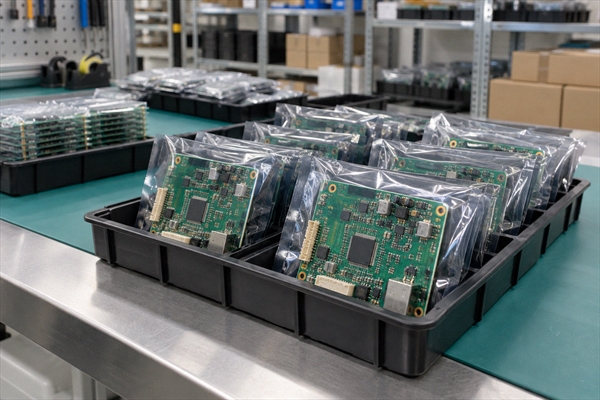
A drawing may use the wording IPC A 600 class II for Class 2. The class, revision and any customer-specific requirements together define what is requested. We can review those requirements against your stack-up and features before manufacture; assigning a class alone does not establish every material, construction or test requirement.

How Does IPC-A-600 Relate to IPC-6012 and IPC-A-610?

IPC-A-600 helps interpret observable board conditions, while the applicable performance specification defines requirements for the board construction. IPC A 600 vs IPC 6012 is therefore a comparison of complementary documents, not two interchangeable inspection options.

Document	Scope	Connection to the product we supply
IPC-A-600	Illustrated acceptability of bare printed boards	A common reference for interpreting visible and sectioned board features.
IPC-6012	Rigid-board qualification and performance requirements	Relevant to specifying rigid PCB fabrication requirements.
IPC-6013	Flexible and rigid-flex board qualification and performance requirements	Relevant to constructions with flexible sections.
IPC-A-610	Acceptance of electronic assemblies	Relevant after components are assembled onto the PCB.

For IPC A 600 vs IPC A 610, the key boundary is bare PCB fabrication versus electronic assembly. We offer both PCB manufacturing and PCB assembly, so these are distinct stages of a project: board acceptance addresses the substrate and circuitry; assembly acceptance addresses the populated product.

Which Bare-Board Features Affect Assembly Quality?

Pads, conductor geometry, holes and solder-mask openings form the interfaces between a bare PCB and the assembly process. Their condition matters because components must fit, intended soldering areas must remain accessible, and conductors must retain the geometry required by the design.

Conceptual view of bare PCB pads, holes and conductor patterns examined with a magnifier

Exposed lands: pad condition and unwanted mask coverage affect the available soldering surface.
Conductor patterns: unwanted copper connections or missing conductor material can change the intended circuit.
Holes and mounting features: finished dimensions affect lead insertion, mounting and mechanical fit.
Board outline and laminate: edge condition and visible material damage can affect handling and fit in the assembly.

Our PCB inspection capabilities include AOI, hole-diameter inspection and dimensional measurement. These methods support different questions: an optical examination locates a visible feature, while a measurement establishes its size or position. For your board, the relevant drawing requirements provide the link between what is observed and what the assembly needs.

What Can Microsection Analysis Reveal Inside Your PCB?

Microsection analysis exposes internal construction that cannot be assessed from a surface photograph. A prepared section can show the relationship between a plated hole, inner-layer copper and the surrounding laminate. That is valuable when the question concerns an interconnection inside the board rather than an exposed pad.

Conceptual PCB microsection showing a plated hole wall and internal copper connections, not to scale

We provide microsection preparation and analysis and copper-thickness testing as part of our PCB testing capabilities. For our HDI boards, the question may involve a microvia interface or an interconnected via structure. The section location and represented construction therefore matter as much as the image itself.

The benefit for your project is evidence about an otherwise hidden feature. A section represents the sampled area; additional sampling or reliability evaluation may be needed for the application’s requirements. The illustration above explains the inspection concept and is not a production micrograph.

How Does Electrical Testing Complement Visual Inspection?

Electrical testing evaluates whether intended nets are connected and separate nets remain isolated under the test conditions. Visual inspection examines physical features. Together they address two different aspects of the bare board: its construction and its circuit connectivity.

Conceptual flying-probe test station contacting separate pads on an unpopulated PCB

Our PCB testing capabilities include flying-probe testing, universal electrical testing and open/short testing. These are directly relevant to finding connectivity faults before components are added. A conductor pattern may appear complete yet contain an open connection; electrical testing addresses that question without relying on appearance alone.

For designs with controlled-impedance traces, we also provide impedance testing. This answers a different question from continuity: whether the specified transmission-line characteristic is achieved. The tests required for a particular board depend on its design and the agreed requirements; an electrical pass is not a substitute for every other specified evaluation.

Why Do Different PCB Constructions Need Different Checks?

Different constructions contain different interfaces and interconnections. The acceptance reference remains useful across them, but the features relevant to a two-layer rigid board are not identical to those in a multilayer HDI or rigid-flex design.

PCB construction	Relevant features	What they mean for your design
FR4 printed circuit boards	Outer patterns, plated holes and the internal connections present in the stack-up	Component mounting and the intended paths between copper layers.
HDI boards	Microvia interfaces and filled or capped vias where specified	Connections that support dense routing and fine-pitch component layouts.
Rigid-flex circuits	Coverlay openings, bonded regions and rigid-to-flex transitions	Electrical connections and the mechanical interfaces involved in installation or flexing.

Our FR4 manufacturing capability extends to 32 layers, subject to the stack-up, dimensions, materials and engineering review. As internal connections become more complex, the construction information becomes more important to selecting meaningful inspection evidence. This is why layer count alone is not enough to describe the board we are being asked to manufacture.

How Can Inspection Evidence Help Resolve a Board Concern?

A useful quality discussion connects the observed condition to the affected feature and its requirement. If you have a concern about a supplied board, we can review it with your part information, the location of the feature and the relevant photographs or measurements. That gives both teams a specific technical issue to discuss.

For example, a question about whether a lead will fit a hole calls for finished-hole dimensions and the component requirement. A concern about an internal connection may call for sectioning or electrical evidence instead. The benefit is a response directed at the actual board function, rather than a general judgment based on one photograph. Any proposed change to an agreed acceptance requirement needs customer agreement.

What Does IPC-A-600 Certification Mean for Customers?

IPC A 600 certification refers to personnel training and assessment credentials. It answers a question about knowledge of the standard, whereas inspection and test results answer questions about a particular board or lot. These are different forms of evidence.

For your project, the relevant discussion with us is the required board construction, acceptance basis and available inspection or testing support. Personnel credentials, when required, need separate confirmation of their scope and validity. A credential is not a replacement for evidence about the product being delivered.

How Can We Support Your Next PCB Build?

We combine custom PCB manufacturing, DFM engineering review and PCB testing support. This lets us discuss your acceptance requirements in the context of the actual board, from its stack-up and holes to its surface finish and assembly interfaces.

For an IPC-A-600 question about your next build, contact sales@bestpcbs.com with your fabrication data and the requirements already defined for the project. At EBest Circuit (Best Technology), we can review the design and discuss the applicable inspection and testing needs before manufacture.

Cleaning Electronics With Rubbing Alcohol: 70%, 90%, or 99% IPA?

September 10th, 2026

Cleaning electronics with rubbing alcohol can be safe when the device is disconnected from power, the liquid is kept out of openings, and the concentration matches the surface. For exposed PCBs, 90% to 99% electronics-grade isopropyl alcohol (IPA) is usually a better starting point than 70% rubbing alcohol because it contains less water and dries faster.

That does not make IPA a universal electronics cleaner. Display coatings, printed legends, adhesives, unsealed sensors, and some plastics may be damaged. The contamination also matters: IPA can lift oils and many rosin-based flux residues, but it may not remove salts, sugary spills, water-soluble flux, or cured residues.

Technician cleaning a powered-off PCB at an ESD-safe workbench with rubbing alcohol

Can You Clean Electronics With Rubbing Alcohol?

Yes, you can clean selected electronics with rubbing alcohol after removing power and confirming that the device maker permits alcohol on the target surface. A slightly damp lint-free cloth may be suitable for an approved hard exterior, while an exposed PCB normally calls for controlled application of 90% to 99% electronics-grade IPA.

First decide which job you are doing:

Exterior wiping: Some manufacturers permit 70% IPA wipes on hard, nonporous surfaces. Apple and Dell publish product-specific examples, but their instructions do not apply automatically to every device.
Exposed-board cleaning: Repair guides commonly use at least 90% IPA for localized work on a disconnected logic board or PCB.
Disinfection: The concentration and wet contact time needed to disinfect a surface are different from the requirements for removing flux or oil from a circuit board.

Never spray alcohol directly onto a device. Wet the cloth, foam swab, polyester swab, or ESD-safe brush away from the electronics, then apply only enough liquid to loosen the soil.

Is Rubbing Alcohol Safe for Electronics?

Rubbing alcohol is safe only for compatible materials and controlled, unpowered cleaning; it is not safe to pour into an assembled device or use around ignition sources. A 70% IPA wipe may be approved for a laptop shell or keyboard, yet the same liquid can enter a connector, remain beneath a shield, soften adhesive, or mark a coated display.

This is why the answer to whether rubbing alcohol is safe for electronics depends on the exact part, contamination, and application method rather than the device category alone.

The label matters as much as the percentage. A bottle sold as first-aid rubbing alcohol is formulated for topical use, not residue-sensitive PCB production. Many 70% products contain 30% water, and formulations vary by supplier. Before use, check the active ingredients, inactive ingredients, and safety data rather than assuming every clear alcohol product is equivalent.

IPA is also highly flammable. NIOSH lists isopropyl alcohol as a Class IB flammable liquid with a 53°F (12°C) flash point. Keep it away from soldering irons, hot-air rework tools, sparks, smoking, and open flame; cap the container when not in use and provide ventilation.

What Percentage Isopropyl Alcohol for Electronics?

Use the device maker’s approved product for finished equipment; for localized exposed-PCB cleaning, 90% to 99% electronics-grade IPA is the practical starting range because it contains only 1% to 10% water instead of the 30% found in 70% IPA. Higher purity does not override component, coating, or adhesive restrictions.

IPA Concentration	Approximate Water Content	Suitable Starting Use	Main Limitation
70%	30%	Approved hard exterior surfaces using a damp wipe	Slower drying and more water; not the default for exposed PCBs
90% or 91%	9% to 10%	Localized PCB repair and residue removal when compatible	Can still affect coatings, plastics, markings, and adhesives
99% or 99.9%	0.1% to 1%	Moisture-sensitive, residue-controlled bench cleaning	Still flammable and not effective against every contaminant

Comparison of 70 percent, 90 percent, and 99 percent IPA for exterior and exposed PCB cleaning

Do not dilute high-purity IPA with tap water for PCB work. Tap water can add minerals and ions. If an aqueous process is required, it should use chemistry, rinse-water quality, and drying conditions chosen for the assembly.

What Is the Difference Between Rubbing Alcohol and Electronics-Grade IPA?

Household rubbing alcohol is usually sold as a skin antiseptic, whereas electronics-grade IPA is supplied with controlled purity and residue expectations for cleaning components and assemblies. A common 70% first-aid product is 70 mL IPA per 100 mL with water as the inactive ingredient; an electronics cleaner may be 99.9% anhydrous IPA with a technical data sheet and safety data sheet.

Do not judge a cleaner by the front label alone. Check:

IPA concentration and water content;
listed fragrance, dye, oil, bitterant, or other additive;
nonvolatile residue specification, if provided;
plastics, elastomer, coating, and adhesive compatibility;
storage, ventilation, and personal-protection instructions in the SDS.

For a repeatable manufacturing process, lot-controlled cleaner and documented compatibility are more useful than a generic pharmacy bottle whose intended use is first aid.

Which Parts Should Not Be Cleaned With Rubbing Alcohol?

Do not apply rubbing alcohol to an unapproved display coating, printed key legend, foam adhesive, acrylic or polycarbonate part, unsealed microphone, speaker, sensor, relay, or coated PCB area without a material check. Even when the bare laminate and solder mask tolerate IPA, a complete assembly may contain liquid-trapping or solvent-sensitive parts.

Display coating, printed legends, adhesive tape, and an unsealed sensor that require IPA compatibility checks

Displays and lenses: Alcohol can affect oleophobic, anti-glare, or other surface treatments unless the manufacturer permits it.
Printed markings: Repeated wiping can fade legends on keys, component bodies, labels, and enclosures.
Adhesives and foam: IPA is often used to weaken adhesive during repair, which is exactly why it must be controlled near display seals, battery tape, gaskets, and foam pads.
Liquid-sensitive devices: Microphones, speakers, MEMS parts, unsealed switches, relays, transformers, and trimmers can trap solvent or suffer mechanical damage.
Conformal coating: Cleaning a coated board and intentionally removing coating are different processes. Review the coating chemistry before applying solvent.

How Should You Prepare Electronics Before Cleaning?

Shut the device down, unplug every cable, remove the battery when serviceable, verify stored energy is discharged, and move the work away from sparks, hot tools, and open flame. A power button does not isolate every energy source, and power supplies or large capacitors may retain hazardous voltage after unplugging.

Read the product cleaning or service instructions.
Photograph connectors, cable routing, corrosion, and residue before disassembly.
Disconnect mains power, external supplies, and batteries.
Use an ESD-safe mat, grounded tools, and an ESD-safe brush for sensitive boards.
Remove loose dust first so wet cleaning does not turn it into a paste.
Test the cleaner on a hidden or representative material when compatibility is uncertain.
Use ventilation and keep the IPA container away from ignition sources.

If you cannot safely discharge the equipment, access the board without damaging seals, or identify a swollen battery, stop and use a qualified repair service.

How Do You Clean an Exposed PCB With Isopropyl Alcohol?

Apply a small amount of 90% to 99% electronics-grade IPA to a low-lint swab or ESD-safe brush, loosen the soil, then lift the dissolved residue with clean material instead of letting dirty solvent dry on the board. The goal is removal, not simply spreading a dissolved film across a larger area.

Controlled cleaning of flux residue from an exposed PCB with a low-lint swab

Inspect and classify the soil. Note whether it is dry dust, oil, flux, drink residue, corrosion, or an unknown deposit.
Remove dry particles. Use an ESD-safe soft brush or controlled clean air without forcing debris under packages.
Dampen the tool. Add IPA to the swab or brush away from the PCB; do not pour from the bottle onto the board.
Agitate gently. Work around solder joints and leads without bending parts or snagging fine wires.
Lift the dissolved residue. Blot with a clean low-lint wipe or use fresh solvent as a controlled final rinse.
Replace dirty materials. A brown swab or cloudy solvent is carrying contamination and should not be reused for the final pass.
Dry, inspect, and test. Confirm that connectors, shields, sockets, and package gaps are dry before reconnecting power.

For a broader method covering dust, corrosion, coating, and aqueous cleaning, see our guide to cleaning a PCB board safely.

Which Contaminants Need More Than IPA?

Salt, sugary drinks, water-soluble flux, corrosion products, and unknown deposits may require a qualified aqueous rinse, flux-specific cleaner, or repair process rather than an IPA-only wipe. IPA can evaporate while nonvolatile ionic contamination stays behind.

Contaminant	Suitable Starting Method	Why IPA Alone May Fail
Finger oil or light grease	Compatible high-purity IPA and clean low-lint material	Dirty solvent can redeposit an oily film
Rosin-based flux	High-purity IPA or matched flux remover after compatibility check	Heat-aged or polymerized residue may resist IPA
Water-soluble flux	Validated aqueous chemistry and DI-water rinse	IPA may not remove the ionic activator system
Sugary or salty spill	Controlled aqueous cleaning, DI rinse, and complete drying when parts allow	Alcohol can leave conductive nonvolatile material behind
Corrosion	Cleaning plus magnified damage assessment and repair	Solvent cannot restore missing copper or damaged terminations

Flux chemistry should be identified before selecting the cleaner. Our explanation of flux residue and cleaning methods shows why water-soluble, rosin, and no-clean materials cannot share one blanket instruction.

In our PCBA projects, we treat cleaner selection, rinse quality, drying, and inspection as one process. Changing only the solvent can leave the same ionic residue or hidden moisture problem in a different form.

How Long Should Electronics Dry Before Power-On?

Do not use one universal minute count; restore power only after visible liquid and alcohol odor are gone and no fluid remains trapped under shields, connectors, sockets, switches, or packages. A lightly wiped open surface may appear dry within minutes, while a flooded connector or shielded area can retain solvent much longer.

Use these release checks:

no droplets, wet sheen, or cleaner line visible under magnification;
no liquid emerging when the board is tilted or gently repositioned;
connectors and sockets inspected from more than one angle;
no alcohol odor at close range in a ventilated area;
no residue film, displaced component, lifted pad, or damaged marking;
the device maker’s minimum drying instruction has been met.

Do not use a hot heat gun to accelerate drying. Excessive heat can deform connectors, soften adhesives, damage batteries, or stress solder joints. Use clean dry air or a controlled low-temperature process only when the component limits are known.

What Mistakes Damage Electronics During Alcohol Cleaning?

The highest-risk mistakes are cleaning an energized device, spraying directly into openings, flooding liquid-sensitive parts, using a contaminated swab, and restoring power before trapped solvent has evaporated. Most failures come from uncontrolled application or wrong-material use, not from the word “alcohol” alone.

Using 70% as the universal choice: It may be suitable for an approved exterior but adds more water to an exposed assembly.
Using a soaked cotton swab: Excess liquid can wick under components, and loose fibers can snag on leads.
Letting dirty IPA evaporate: Dissolved flux and oil remain unless they are lifted or rinsed away.
Scrubbing harder: Force can remove markings, dislodge 0201/01005 components, bend contacts, or break corroded leads.
Ignoring the original fault: Cleaning cannot repair a cracked joint, missing copper, swollen battery, or internally corroded component.
Applying conformal coating over residue: Cleanliness and dryness must be verified before coating, or contamination may be sealed onto the assembly.

Production control begins earlier than final cleaning. For example, solder paste inspection in PCB assembly can catch printing defects before placement and reflow, while post-solder cleaning addresses only the residue left by the selected materials and process.

FAQ About Cleaning Electronics With Rubbing Alcohol

These answers cover the most common concentration, surface, flux, and power-on questions about using rubbing alcohol on electronics.

Can I use 70% rubbing alcohol on a circuit board?

Use 70% rubbing alcohol on an exposed circuit board only when the assembly documentation permits it and no better high-purity option is available. Its 30% water content slows drying and raises the chance of liquid remaining in gaps. For localized exposed-PCB cleaning, 90% to 99% electronics-grade IPA is usually the safer starting range.

Is 91% rubbing alcohol good for electronics?

91% IPA is suitable for many localized PCB-repair tasks because it contains about 9% water and evaporates faster than 70%. It can still soften adhesive, affect markings, or enter unsealed parts, so apply a small amount to a low-lint tool and check material compatibility first.

Can I use 99% isopropyl alcohol on a phone screen?

Do not use 99% IPA on a phone screen unless the phone manufacturer explicitly approves it for that model and surface. Screen coatings and display seals vary. Many device makers specify a slightly damp lint-free cloth or a 70% IPA wipe for selected exterior surfaces, not unrestricted use of 99% liquid.

Does isopropyl alcohol remove solder flux?

IPA removes many fresh rosin-based flux residues, especially at 91% to 99%, but it does not remove every no-clean or heat-aged residue. Water-soluble flux normally requires a validated aqueous process. Match the cleaner to the exact flux product and remove the dissolved soil rather than letting it dry on the PCB.

Can cleaning electronics with alcohol cause a short circuit?

Cleaning electronics with alcohol can cause a short circuit if power is present, the liquid contains conductive contamination, or water and dissolved residue remain trapped when the device is energized. Disconnect every power source, control the liquid, dry hidden areas, inspect the board, and only then perform a safe functional test.

Can I pour rubbing alcohol over a motherboard?

Do not pour household rubbing alcohol over an assembled motherboard. Flooding carries dirt beneath packages and into connectors, fans, sockets, microphones, switches, or other liquid-sensitive parts. Board immersion is a specialized repair process that requires disassembly, compatible components, suitable high-purity solvent, ventilation, and controlled drying.

How Can EBest Circuit Support Cleaner, More Reliable PCB Assemblies?

We match the cleaning method to the flux, component set, coating plan, inspection requirement, and end-use risk instead of treating IPA as a universal production solution. At EBest Circuit, we support PCB fabrication, component sourcing, PCB assembly, and inspection within one coordinated project.

For a cleaning-sensitive assembly, send us the Gerber files, BOM, placement data, assembly drawing, target flux or solder-paste specification, coating requirement, quantity, and cleanliness or test criteria. We can review the build information before production and align the inspection plan with the assembly design.

To discuss a PCB or PCBA project, visit our PCB and PCBA manufacturing service page or email sales@bestpcbs.com.

Why Does AI Computing Hardware Use Advanced HDI PCBs?

September 9th, 2026

Advanced HDI PCBs become necessary when dense accelerator I/O, fast board-level links, multiple power rails, and cooling hardware compete for the same board area. Fine-line routing, laser-drilled microvias, filled via-in-pad, and selective build-up layers create escape and transition paths that conventional through-hole vias can block.

That pressure is rising in 2026. NVIDIA Rubin, AMD Helios, and new 102.4 Tbps switch silicon show AI systems moving toward more accelerator bandwidth, larger scale-up domains, denser networking, and tighter power-and-cooling integration. At board level, the practical result is more difficult package breakout, more high-speed lanes, heavier power distribution, and less room to solve them.

advanced HDI PCBs, white-background AI accelerator board beside an exploded multilayer HDI structure

Why Does AI Computing Hardware Need Advanced HDI PCBs?

AI hardware needs advanced HDI when the package map and board outline leave too few routing channels for ordinary through-hole construction. The important gains are specific:

advanced HDI PCBs, three-dimensional BGA escape cutaway with via-in-pad and blind microvia connections

Dense BGA escape: Blind microvias move power, ground, control, and high-speed signals away from fine-pitch accelerator or switch packages without reserving a through-hole barrel on every layer.
More usable routing channels: Smaller pads and layer-specific vias leave inner-layer space for differential pairs, clocks, control buses, and power connections.
Shorter vertical transitions: A microvia can reach the required reference or signal layer without the long unused barrel of a full-depth via.
Local power access: Via-in-pad and short power-ground transitions help connect dense decoupling and nearby regulators to high-current devices with less interconnect inductance.
Room for the rest of the system: Routing density preserves surface area for retimers, connectors, stiffeners, cold-plate hardware, test points, and service clearances.

A low-speed management board or power-only board may not need this construction. The trigger is a verified routing, signal, power, or space constraint on the actual board.

Where Are Advanced HDI PCBs Used in AI Computing Hardware?

Advanced HDI is most useful on boards where fine-pitch packages and dense local interconnects occupy the same limited area:

GPU and AI accelerator cards: Microvias and via-in-pad help escape large accelerator packages, memory-adjacent board interfaces, retimers, clocks, and dense local power connections.
Accelerator modules and baseboards: High connector counts, scale-up links, switch devices, and management circuits compete for routing and reference-plane space.
AI server PCBs and motherboards: Selective HDI can relieve congestion around CPUs, high-speed I/O hubs, PCIe or CXL devices, NICs, and module connectors without forcing advanced rules across the whole board.
AI network and switch boards: Very large switch ASICs, dense SerDes fan-out, retimers, and pluggable-module connectors create concentrated breakout and transition problems.
Edge AI compute modules: A small outline must accommodate an AI SoC, memory, PMICs, cameras, storage, sensors, radios, and external I/O, making area efficiency the main driver.

These boards can sit in the same AI system and still require different constructions. An accelerator module may need local high-density build-up, while a long-channel switch board may depend more heavily on low-loss material, backdrilling, and connector-launch control.

How Does Advanced HDI Support GPU and AI Accelerator Boards?

The main job is package breakout. Large GPU, ASIC, and FPGA packages bring thousands of power, ground, clock, control, and high-speed connections into a compact footprint. Conventional capture pads and antipads can close routing channels before those connections reach usable signal and plane layers.

Blind microvias open escape paths by connecting only the layers needed around the package.
A filled and capped via-in-pad structure removes the dog-bone penalty where the land pattern leaves no room for a separate fan-out via.
Selective build-up keeps aggressive geometry local to the accelerator, retimer, or module-connector region instead of applying it to every route.
Short local transitions reduce congestion between the accelerator and nearby switches, retimers, NICs, CPUs, clocks, and power stages.

The safest design uses the coarsest feature that still closes the breakout. Finer lines, smaller pads, and more stacked microvia levels increase registration, plating, planarization, inspection, and yield demands.

Why Do AI Accelerator Boards Use High-Layer-Count HDI Stackups?

AI accelerator boards push layer counts higher because package breakout, high-speed channels, continuous reference planes, multiple power rails, and connector fan-out all need separate space in the same cross-section. Combining high layer count with selective HDI lets the board assign each constraint to a controlled part of the stack.

Breakout and build-up layers move dense package connections out of the BGA field before the routes spread across the board.
High-speed signal layers carry PCIe, scale-up, network, clock, and control paths beside stable reference planes.
Reference planes give fast signals a continuous return path and reduce coupling between unrelated channel groups.
Power-distribution layers connect regulators, planes, and decoupling to high-current loads while keeping loop inductance under control.
Connector and long-channel layers reserve cleaner routing corridors for paths that cannot tolerate repeated layer changes or plane discontinuities.

This is why a high-multilayer HDI PCB can be useful in an accelerator or baseboard: it separates jobs that would otherwise fight for the same routing space. The final layer count should come from the completed escape study, channel plan, PDN model, board thickness, and fabricator review.

How Does Advanced HDI Support High-Speed Interconnects in AI Hardware?

Advanced HDI supports high-speed board links by controlling how signals leave dense packages and reach a continuous routing layer.

Shorter via barrels reduce unused-stub effects on local transitions where a blind microvia can replace a full-depth plated through hole.
More escape channels reduce route detours, helping differential pairs reach retimers, switches, CPUs, NICs, or module connectors without unnecessary length.
Closer reference access improves return-path continuity when the via transition includes the required ground stitching and keeps plane openings under control.
Selective transitions preserve long-channel options: the dense breakout can use HDI while longer routes use low-loss material, controlled impedance, and backdrilled through vias where those choices provide better margin.

HBM bandwidth is evidence of rising compute density, but HBM traffic between the GPU die and memory stacks stays inside the package and package substrate. The host PCB carries package or module I/O such as scale-up links, PCIe, networking, clocks, control, power, and connector transitions. Simulation should model the channel the PCB actually owns.

Why Do AI Network and Switch Boards Need High-Density Interconnects?

AI switch boards concentrate an unusually large number of SerDes lanes around one switch ASIC. Broadcom announced in March 2026 that Tomahawk 6 was shipping in production volume with 102.4 Tbps switching capacity and support for 100G and 200G SerDes. That scale increases the number of package escapes, reference transitions, retimer connections, and front-panel links a board must organize.

ASIC breakout is the local HDI problem: fine-pitch balls and a large lane count require many short, controlled escapes close to the switch package.
Pluggable optics create a connector-density problem: OSFP or similar cages, management devices, power, and thermal clearances compete for the board edge.
Long routes remain a channel problem: low-loss laminate, trace geometry, connector launches, backdrilling, and return-path design may matter more than microvias once the signal leaves the congested ASIC region.
Retimers change the partition: placing them near the ASIC or front panel trades routing distance against power density, cooling access, and additional BGA escape.

The design decision is regional. Use advanced HDI where it clears the switch or connector breakout, then select the long-channel construction from the measured insertion-loss, crosstalk, and via-stub budget.

How Does Advanced HDI Support Compact Edge AI Modules?

Edge AI modules use HDI primarily to fit more functions into a fixed, often irregular outline. A single board may combine an AI SoC, memory, PMICs, storage, camera inputs, sensors, radios, USB, Ethernet, and board-to-board connectors.

Via-in-pad releases component area around fine-pitch SoCs, memories, and PMICs.
Blind microvias protect inner-layer routing space that a field of through holes would consume.
Short fan-out supports compact high-speed interfaces between the processor, memory, storage, cameras, and communications devices.
Selective build-up controls cost by limiting the most demanding rules to dense device regions.
Smaller transition fields leave room for mechanical needs such as shields, antennas, mounting holes, thermal interfaces, and sealed-enclosure clearances.

Compact does not automatically mean advanced HDI. A board with relaxed pitch, few high-speed interfaces, and enough area may meet its targets with standard multilayer construction. An escape study should show blocked routes or excessive board area before the HDI stack is approved.

How Does Advanced HDI Affect Power and Thermal Design Around AI Accelerators?

Advanced HDI changes power and thermal design by concentrating copper and components while freeing some surface area for regulators and cooling hardware.

Power delivery: Short via-in-pad and microvia connections can reduce the inductive path between package lands, decoupling, and nearby power or ground planes.
Regulator placement: Denser breakout may create usable surface area for multiphase stages, inductors, bulk capacitance, current sensing, and control circuits close to the load.
Heat spreading: Copper planes and via fields alter lateral and vertical heat flow, so conductor losses and component heat must be solved with the real copper distribution.
Warpage and stress: Uneven copper, multiple build-up layers, large packages, stiffeners, and cold-plate fasteners can produce local bending or interface stress during lamination, reflow, and service.
Cooling clearances: Cold plates, retention hardware, liquid manifolds, airflow paths, and service access impose keep-outs that reduce the routing area HDI is trying to recover.
Qualification: Thermal cycling, assembly exposure, cross-sections, resistance monitoring, and representative coupons must match the released microvia structure and material set.

The board should be reviewed with the same stackup in the signal, power, thermal, mechanical, and fabrication models. A routing solution that closes electrically but moves copper or fasteners into the wrong thermal-mechanical condition is not ready for production.

What Do 2026 AI Hardware Platforms Reveal About Future PCB Requirements?

Three 2026 announcements show where board-level pressure is increasing:

NVIDIA Rubin: NVIDIA lists up to 22 TB/s of HBM4 bandwidth per GPU, 3,600 GB/s of NVLink 6 scale-up bandwidth, PCIe Gen 6 host connectivity, and a rack architecture that integrates compute, networking, liquid cooling, and power controls in its Rubin architecture disclosure. For PCB teams, the relevant pressure is dense module I/O, switch and retimer fan-out, power delivery, and cooling-constrained placement.
AMD Helios: AMD describes Helios as a rack-scale system combining Instinct MI455X GPUs, EPYC CPUs, Pensando networking, and ROCm software. The board-level implication is tighter co-design among accelerator modules, baseboards, host processors, network fabrics, power shelves, and serviceable trays.
Broadcom Tomahawk 6: A 102.4 Tbps switch with 100G and 200G SerDes increases the density around the switch ASIC and front-panel interfaces. Local HDI escape, long-channel loss control, retimer placement, and connector launches must be planned as one path.

The next step for high-layer-count HDI PCB design is more selective use of density. Build-up layers will concentrate around accelerators, switches, and connectors; long routes will be assigned by loss and return-path budgets; power and cooling constraints will enter the stackup earlier; and qualification coupons will be designed with the board rather than added after routing.

What Are the Limits of Advanced HDI in AI Hardware?

Advanced HDI is limited by the board constraint it can solve and by the process margin available at the chosen factory.

It cannot fix a weak channel plan: Microvias do not compensate for poor reference continuity, unsuitable laminate, excessive route length, bad connector launches, or missing return vias.
It adds sequential-lamination risk: Every build-up cycle adds registration, drilling, plating, filling, planarization, inspection, and schedule demand.
Stacked microvias require construction-specific evidence: Interface quality depends on via geometry, material, plating, target pads, thermal history, and process control.
Fine features can reduce yield: Small annular structures, narrow conductors, dense via fields, and large panels leave less margin for imaging, etching, and registration variation.
Inspection and rework become harder: Hidden via structures and dense BGAs need planned coupons, electrical tests, X-ray or cross-section checks, and realistic repair limits.
Factory capability is not interchangeable: Materials, panel limits, via spans, fill processes, inspection methods, and qualified build-up sequences vary by plant.
Some boards need a different solution: Power-only and management boards may use standard multilayer construction, while long-channel network boards may gain more from low-loss material and backdrilling than from full-board HDI.

Approve the stackup only after the fabricator returns the actual dielectric, finished copper, via spans, fill and cap process, panel limits, impedance model, coupons, and acceptance plan for the released design.

FAQs About Advanced HDI PCBs for AI Computing Hardware

Q1: Are stacked microvias always better than staggered microvias?

A1: No. Stacking saves routing area but adds plated interfaces in the vertical path. Choose stacked or staggered construction from pad space, routing need, material behavior, fabricator process, and the qualification plan for that exact structure.

Q2: Can standard FR-4 be used for an AI accelerator board?

A2: Sometimes, but FR-4 names a broad material class rather than a complete channel solution. Select laminate from the actual loss, temperature, CAF, thickness, registration, and supply requirements. Local links and long connector channels may need different loss classes within the same platform.

Q3: What should be sent for an advanced HDI manufacturing review?

A3: Send the board outline, BGA maps, proposed stackup, via table, microvia spans, controlled-impedance list, material and copper requirements, fabrication data, assembly constraints, quantities, test scope, and target date. Ask for a returned production stackup and written DFM findings.

Q4: How should an advanced HDI PCB be qualified before volume production?

A4: Use representative coupons, cross-sections, impedance measurements, electrical tests, assembly thermal exposure, and any product-specific reliability tests. Keep the lot, material, process, coupon, and results tied to the same stackup and revision.

Q5: Can the same advanced HDI design move between PCB factories without requalification?

A5: A data package can move, but process capability and material availability may change. Require the receiving factory to return its stackup, impedance model, via process, panel plan, coupon design, and acceptance evidence before release. Requalify any change that affects the product's approved risk controls.

Q6: Can co-packaged optics replace advanced HDI in AI systems?

A6: Co-packaged optics can shorten some electrical paths, yet the optical engine still needs dense power, control, thermal, mechanical, and short electrical connections. It changes where the interconnect problem sits; it does not remove board-level density.

Advanced HDI PCBs are justified when they remove a measured bottleneck in accelerator, server, switch, or edge hardware. Start with the package maps, interface list, PDN targets, board outline, cooling keep-outs, and channel budgets; then use the least complex stackup that closes those constraints with manufacturing margin.

For a project-specific review, send EBest Circuit your Gerber or ODB++ data, board outline, proposed stackup, microvia map, impedance requirements, materials, copper weights, BOM, quantity, test scope, and target schedule. Our engineering team can perform a free DFM review and return the fabrication questions that affect manufacturability, cost, and lead time. Email sales@bestpcbs.com to request an advanced HDI PCB or PCBA quotation.

What Are Embedded Systems? Components, Examples and PCB Design

September 8th, 2026

What are embedded systems? They are purpose-built computers integrated into products or machines to monitor inputs, make decisions, and control specific functions. An embedded system combines electronic hardware with firmware or software, and it is normally designed around limits such as response time, power, size, operating environment, and cost.

A simple thermostat and a multi-board industrial controller can both be embedded systems. Their complexity differs, but the design question is the same: can the hardware and software perform the required function predictably inside the finished product?

Embedded control PCB connecting a sensor input to a motor output

What Is an Embedded System?

An embedded system is a computer built into a larger product to perform a defined function or a limited group of related functions. It may be nearly invisible to the user, yet it can control sensing, communication, motion, power conversion, safety monitoring, or a user interface.

The word “embedded” describes the system’s role, not a particular processor or board size. A design may use an 8-bit microcontroller, a 32-bit MCU, a microprocessor running embedded Linux, an FPGA, or a system-on-chip. What makes it embedded is that its computing resources are selected and programmed for the product rather than for unrestricted general-purpose use.

How Does an Embedded System Work?

Most embedded systems follow an input-process-output loop. Sensors, switches, or communication interfaces provide input; the processor runs control logic; outputs then operate a display, relay, motor, valve, radio, or another subsystem.

Input: A sensor, user control, or data interface supplies information.
Signal conditioning: Analog front ends, filters, level shifters, or protection circuits prepare the signal.
Processing: Firmware reads the input, applies rules or algorithms, and decides what should happen.
Output: Driver circuits translate the processor’s low-power signal into a usable electrical or mechanical action.
Feedback: The system checks the result and corrects its next action when closed-loop control is required.

Sensor connected to an embedded control PCB that drives a motor and indicator

What Are the Main Components of an Embedded System?

An embedded system needs more than a processor. The complete hardware platform must provide stable power, memory, timing, interfaces, protection, and a physical PCB that connects every function.

Processor: An MCU, MPU, DSP, FPGA, or SoC executes the application.
Memory: Flash or other nonvolatile memory stores code; RAM holds temporary data.
Power circuitry: Regulators, filters, supervisors, and protection devices create stable supply rails.
Clock and reset: Oscillators, crystals, reset circuits, and watchdogs control startup and timing.
Inputs and outputs: GPIO, ADC, DAC, sensor interfaces, drivers, displays, and actuators connect computation to the physical world.
Communication: UART, SPI, I2C, CAN, USB, Ethernet, and wireless modules exchange data where the application requires them.
PCB and connectors: The board provides electrical interconnection, grounding, mechanical support, test access, and thermal paths.

An MCU often integrates the processor, memory, timers, ADCs, and common peripherals into one device. An MPU usually depends on external memory and may support a richer operating system. For a practical selection comparison, see our guide to microcontrollers versus microprocessors.

What Are Some Examples of Embedded Systems?

Embedded systems appear anywhere a product must sense, decide, communicate, or control without acting like a conventional desktop computer.

System Example	Typical Input	Processing Task	Typical Output
Washing machine controller	Door, water-level, and temperature sensors	Run the selected cycle and safety interlocks	Valves, heater, pump, and motor
Industrial motor controller	Speed command and current feedback	Control speed, torque, and fault response	Gate-driver or inverter commands
Smart sensor node	Temperature, pressure, motion, or light	Filter readings and package data	Local alarm or network message
Portable monitor	Sensor and user-button inputs	Calculate and record measurements	Display, storage, and alerts
Vehicle control module	Network messages and local sensors	Apply control and diagnostic logic	Actuator commands and status data

The exact architecture depends on consequences of failure, response time, environmental exposure, power budget, service life, and the interfaces shared with the rest of the product.

What Types of Embedded Systems Are Common?

Embedded systems can be grouped by how they operate, but the categories often overlap. A battery-powered IoT sensor, for example, is both portable and networked.

Standalone systems perform their function locally without a continuous network connection.
Networked systems exchange data with other controllers, gateways, servers, or cloud services.
Real-time systems must produce a correct response within a defined timing window; missing the deadline can be as serious as producing the wrong value.
Portable and battery-powered systems prioritize low-power states, efficient conversion, compact packaging, and controlled wake-up behavior.
Safety- or mission-related systems add requirements for fault detection, redundancy, diagnostics, controlled changes, and documented verification according to the application’s governing requirements.

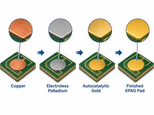
“Real-time” does not simply mean fast. It means the timing behavior is bounded and appropriate for the task. Likewise, not every embedded system needs an operating system; simple controllers can run a loop, state machine, and interrupt handlers directly on the hardware.

How Do Embedded Systems Differ from General-Purpose Computers?

An embedded system is optimized for a defined product function, while a general-purpose computer is built to run many user-selected applications. That difference changes the hardware, software, interfaces, and validation plan.

Design Area	Embedded System	General-Purpose Computer
Primary role	Dedicated product or control function	Broad user-selected computing tasks
Hardware	Selected for a defined workload and environment	Standardized for flexibility and expansion
Software	Firmware, RTOS, or embedded OS tied closely to hardware	Full operating system and replaceable applications
User interface	May be minimal or absent	Usually includes rich user input and display
Validation	Checks the complete product function and interfaces	Emphasizes platform and application compatibility

The boundary is not always sharp. A single-board computer can be used as a general development platform, then become part of an embedded product when its hardware and software are fixed around a specific application.

What Is the Difference Between Embedded Systems and IoT?

An embedded system performs local computing inside a device; an IoT device adds connectivity and normally participates in a wider data or service architecture. Every IoT endpoint contains embedded computing, but many embedded systems are not connected to the Internet.

A motor controller that regulates speed over a local feedback loop is an embedded system. Add a network interface, device identity, secure update path, gateway or cloud connection, and remote data service, and the product may become part of an IoT system. The extra connectivity changes power demand, memory use, cybersecurity planning, radio or Ethernet layout, regulatory work, and lifecycle support.

Embedded controller PCB installed in an industrial automation cabinet

How Does Embedded Software Control the Hardware?

Embedded software configures the processor and peripherals, reads inputs, schedules work, handles faults, and drives outputs. It is usually closer to the hardware than desktop application software because register settings, interrupts, timing, memory limits, and electrical interfaces directly affect behavior.

A small controller may use bare-metal firmware with a main loop and interrupt service routines. A more complex design may use a real-time operating system to schedule tasks and manage communication, or embedded Linux when the product needs extensive networking, storage, graphics, or application frameworks. The most suitable option depends on timing, memory, boot time, update strategy, security, maintainability, and available engineering resources.

Which PCB Design Decisions Matter in Embedded Hardware?

PCB layout turns the system architecture into physical hardware, so electrical, thermal, mechanical, and test requirements must be resolved together rather than after routing.

Power integrity: Place regulators, bulk capacitance, and high-frequency decoupling around the actual load and current path.
Ground and return paths: Give clocks, buses, converters, radios, and analog signals continuous, controlled return paths.
Signal integrity: Treat fast edge rates, not only clock frequency, as the trigger for impedance, termination, crosstalk, and via-stub review.
Analog and digital interaction: Control noisy switching currents before separating areas mechanically or cutting ground planes.
Protection and interfaces: Put ESD, surge, filtering, isolation, and level translation where the external connection enters the board.
Thermal behavior: Estimate loss in processors, regulators, drivers, and power devices, then provide copper area, thermal vias, airflow, or a heatsink path as needed.
Debug and production access: Reserve programming headers or pads, test points, boot controls, and serial diagnostics before the enclosure removes access.
Manufacturability: Review package geometry, component spacing, assembly side, panelization, fiducials, inspection access, and component lifecycle before release.

A control board article can help translate these system requirements into board functions, while our embedded boards guide covers the board-level platform in more detail.

How Should an Embedded System Be Tested?

Testing should prove both that the PCB was assembled correctly and that the complete hardware-software system performs its intended function. A visually perfect board can still fail because of power sequencing, firmware, timing, communication, sensor calibration, or interaction with the enclosure.

Pre-power checks: Inspect polarity, orientation, soldering, resistance to ground, and expected rail isolation.
Controlled power-up: Use current limits and verify each rail, reset state, clock, and boot condition.
Programming and interface checks: Confirm the debug path, firmware image, memory, communication ports, and peripheral identification.
Functional tests: Apply representative inputs and confirm outputs, timing, fault handling, and recovery behavior.
Production coverage: Combine appropriate inspection and electrical methods, which may include AOI, X-ray for hidden joints, in-circuit or flying-probe checks, and a product-specific functional fixture.
System validation: Verify the assembled product under the environmental, electrical, mechanical, safety, EMC, and cybersecurity requirements that apply to its market and use case.

Engineer probing an embedded system PCB during oscilloscope testing

For a closer look at choosing coverage rather than relying on a single inspection step, see our guide to PCB assembly testing services.

FAQ About Embedded Systems

What are embedded systems examples? Common examples include appliance controllers, smart sensors, motor drives, vehicle control modules, printers, cameras, access-control devices, routers, portable instruments, and industrial monitoring equipment. The embedded computer is usually one subsystem inside the finished product.

What are embedded systems and why are they important? Embedded systems give products local sensing, decision-making, communication, and control. They can respond without sending every action to a remote computer, and their hardware can be tailored to the product’s power, size, cost, and environmental limits.

What are embedded systems in IoT? In an IoT product, the embedded system reads sensors, controls local functions, manages a communication interface, and prepares data for a gateway or cloud service. Secure identity, updates, data protection, and loss-of-network behavior become part of the design.

What are embedded systems in electronics? They are electronic assemblies that combine processing, memory, power, I/O, and firmware to perform a defined function. The processor may be a microcontroller, microprocessor, SoC, DSP, or FPGA, depending on the workload.

Do all embedded systems use an RTOS? No. A simple controller can run a loop, state machine, and interrupts without an operating system. An RTOS becomes useful when several time-sensitive tasks, communication stacks, resource sharing, or maintainable scheduling justify the added software layer.

Is a Raspberry Pi an embedded system? It can be. The board is a general development platform, but it becomes part of an embedded system when it is integrated into a product with a fixed function, controlled software image, defined interfaces, and a product-level validation plan.

How Can EBest Circuit Help Turn an Embedded Design into Hardware?

The practical answer to what are embedded systems is that hardware and software must work as one product. At EBest Circuit, we support PCB design review, prototyping, PCB fabrication, component sourcing, PCBA assembly, and testing for teams turning embedded designs into physical assemblies.

For an engineering review or quotation, send your Gerber files, BOM, quantity, assembly drawings, and available programming or functional-test requirements to sales@bestpcbs.com. We can review the manufacturing package and help identify PCB or assembly details that should be resolved before production.

How to Differentiate Between Direct Current and Alternating Current?

September 7th, 2026

To differentiate between direct current and alternating current, determine whether the current keeps flowing in one direction or reverses direction over time. Direct current (DC) is unidirectional and normally keeps fixed polarity. Alternating current (AC) reverses direction periodically, so its polarity alternates.

Direction is the deciding property, while source markings, waveform shape, frequency and meter readings provide supporting evidence. This distinction matters because a changing voltage is not automatically AC, and a DC supply does not have to produce a perfectly flat line.

differentiate between direct current and alternating current, AC and DC power conversion board on a laboratory bench with waveform display

How Can You Differentiate Between Direct Current and Alternating Current?

Start with current direction, then confirm the result from polarity, waveform, source markings and an appropriate measurement. This provides a reliable way to differentiate between direct current and alternating current. Work at a named pair of terminals or test points because the input and output of the same device may use different current types.

Define the measurement point: Identify the two terminals and the expected voltage range. This prevents an AC input and a DC output from being treated as one source.
Check direction and polarity: Current that stays unidirectional, with the same terminal remaining positive relative to the other, is DC. Periodic reversal of direction and polarity identifies AC.
Read the waveform: A trace that repeatedly crosses its reference in both directions is AC. A varying trace that remains on one side is DC or pulsating DC, even when it has a repeating shape.
Read the source markings: Look for V⎓, V~, a polarity diagram and separate input and output ratings. Treat the voltage number as magnitude information, not as proof of AC or DC.
Confirm with a suitable measurement: Compare DC-voltage and AC-voltage readings using equipment rated for the circuit. A result in both modes can indicate DC with ripple or an AC waveform with a DC offset, so interpret both readings at the same test point.

A “12 V” marking alone does not answer the question. It could describe a battery, a 12 V DC adapter output or a 12 V AC transformer secondary. The unit gives the voltage level; the symbol and polarity information identify the current type.

Why Are Direction and Polarity the Defining Differences Between AC and DC?

AC and DC are classified by how charge flow behaves over time. In a DC circuit, conventional current continues through the circuit in one direction. In an AC circuit, the driving voltage reverses polarity, causing conventional current in a resistive load to reverse as well.

Polarity provides a practical way to observe that direction. A DC source normally keeps the same terminal positive relative to the other terminal. An AC source makes each terminal alternate between positive and negative relative to the other. The voltage magnitude may change in either system, so magnitude alone does not define AC or DC.

Characteristic	Direct current (DC)	Alternating current (AC)
Direction	Charge flow remains unidirectional, although its magnitude may rise or fall	Charge flow reverses direction at repeating intervals
Polarity	The same terminal normally remains positive relative to the reference	Each terminal alternates between positive and negative relative to the other
Voltage over time	May be steady, slowly changing or pulsating without crossing the reference	Changes sign relative to the reference as polarity reverses
Typical waveform	Flat level, sloping level or one-sided pulses; ripple may ride on the DC level	Sine, square, triangular or distorted waveform that alternates between polarities
Frequency	Steady DC is 0 Hz; ripple or switching noise can add periodic components	Has an alternating frequency, such as 50 or 60 Hz for utility power
Typical notation	V⎓, DC, or a solid line above a dashed line; polarity may be marked + and −	V~, AC, a tilde or a sine-wave symbol; frequency may also be stated
Practical confirmation	DC mode shows the main level and polarity; reversing the probes reverses the sign	AC mode shows the alternating component; an oscilloscope confirms repeated polarity reversal

Frequency supports the classification but does not replace the direction test. Ripple on a DC rail has a frequency, yet the rail remains DC if its overall polarity does not reverse. This is why direction and polarity come before frequency when the result is uncertain.

What Do AC and DC Waveforms Look Like?

A DC waveform remains on one side of the zero reference, whereas an AC waveform alternates across the reference. A flat DC line and a sine-wave AC trace are familiar examples, but waveform shape by itself is not the definition.

differentiate between direct current and alternating current, AC and DC waveforms comparing a one-polarity DC trace with a polarity-reversing AC trace

Steady DC: The trace appears as a flat horizontal level because magnitude and polarity remain constant. A battery that slowly falls in voltage during discharge is still DC because its direction does not reverse.
Pulsating DC: The trace repeatedly rises and falls while remaining on one side of the reference. An unfiltered rectifier output is a common example: it varies with time but remains unidirectional.
Sine-wave AC: The trace moves smoothly above and below the reference, so its polarity and current direction reverse during every cycle.
Nonsinusoidal AC: Square, triangular and distorted traces change shape differently, but they are still AC when they repeatedly alternate between positive and negative polarity.

On a real measurement, the zero reference must be defined correctly. A waveform may appear to sit above zero because it carries a DC offset even though an AC component is present. That mixed case is addressed separately below.

How Can You Tell Whether a Voltage Is AC or DC With a Multimeter?

Identify the test point and expected range, then measure the same two points in DC-voltage and AC-voltage modes. DC mode reports the average level and polarity; AC mode reports the alternating component within the meter’s bandwidth. Comparing the two prevents ripple or DC offset from being mistaken for a single current type.

Identify the circuit and test point: Read the source label, choose the exact terminal pair and estimate the maximum voltage. The input and output of a charger, inverter or power supply may require different settings.
Verify the meter setup: Confirm that the meter, probes and measurement category are rated for the circuit, and place the leads in the correct sockets. Start on a higher range if the value is uncertain. Do not probe live mains unless you are qualified and equipped to do so.
Measure in DC-voltage mode: Select V⎓ and connect the probes across the test points. A stable positive value shows the red probe is at the more positive point; a stable negative value usually means the probes are reversed. A value that changes but keeps the same sign can still be DC.
Measure the same points in AC-voltage mode: Select V~ without moving the test points. A substantial reading indicates an alternating component, but the displayed value depends on the meter’s bandwidth, waveform response and AC-coupling method.
Compare the two results: A battery should show its main value in DC mode and little AC apart from noise or ripple. A transformer secondary should show its main value in AC mode. A regulated DC supply with measurable AC usually contains ripple rather than having changed into an AC source.
Resolve an ambiguous result: If both readings are significant, check the circuit documentation and observe the waveform with a properly rated oscilloscope. Confirm whether the signal crosses the reference, carries a DC offset or contains switching pulses before assigning the final classification.

A nonzero reading in both modes does not automatically mean the meter is wrong. It may indicate DC with ripple, an AC signal with DC offset, electrical noise or a measurement limitation. Interpret the reading at the exact test point rather than assigning one current type to the entire device.

Which Common Power Sources Provide AC and Which Provide DC?

Batteries, USB ports and photovoltaic panels normally provide DC, while wall outlets, alternators and conventional transformer secondaries normally provide AC. Conversion equipment can make the input and output different, so always identify the side of the device being discussed.

Batteries and cells: These provide DC with defined positive and negative terminals. Their voltage can fall with discharge and load without changing the classification.
USB and regulated electronic outputs: These provide DC at a specified nominal voltage. Switching ripple may be present on the output.
Photovoltaic panels: Individual panels generate DC. A solar inverter converts that DC into AC for conventional AC loads or grid connection.
Household wall outlets: These provide AC at the local utility voltage and frequency. Appliances often convert it to DC internally.
Generators and alternators: Their electrical output is commonly AC. A rectifier may be added when the connected system requires DC.
Transformer secondaries: A conventional transformer changes an AC voltage level but still produces AC. A complete wall adapter adds rectification and regulation to provide DC.

The source category is a useful clue, not a substitute for reading the terminals. An inverter receives DC but delivers AC. A phone charger receives AC at its wall input and delivers DC at its USB output.

Can AC and DC Exist in the Same Circuit at the Same Time?

Yes. One device can contain separate AC and DC sections, and one conductor can carry a DC level with an AC component superimposed on it. The correct description depends on the test point and the purpose of the measurement.

A nominal 5 V DC rail may carry 50 mV peak-to-peak switching ripple. The 5 V average level is the DC component, while the repeating variation is the AC component. The rail is still called a DC supply because its polarity remains fixed and the DC level supplies the load.

Biased audio and sensor circuits provide another example. The signal may swing above and below a DC bias voltage without crossing the circuit’s zero reference. AC coupling can remove the DC component for analysis, while DC coupling shows the combined waveform.

A power adapter contains both forms at different locations: AC at the input, pulsating DC after rectification and smoother DC after filtering and regulation. Identifying the current type therefore requires a test-point reference, not a label applied to the whole product.

How Is AC Converted to DC and DC Converted to AC?

A rectifier converts AC to DC, and an inverter converts DC to AC. Filtering and regulation are normally added when the next circuit needs a controlled voltage rather than the raw converted waveform.

differentiate between direct current and alternating current, engineering diagram showing how AC is converted to DC through rectification and filtering and how DC is converted to AC through inversion

Rectifier, AC → DC: Diodes or controlled switches make the output unidirectional. A reservoir capacitor reduces the variation, and a regulator can hold the output closer to its target.
Inverter, DC → AC: Power switches reverse the output polarity in a controlled sequence. The switching pattern and filtering determine the resulting AC waveform.
DC-DC converter, DC → DC: A switching stage raises, lowers or isolates a DC voltage to create another DC rail. Internal switching does not make the final output AC when its polarity remains fixed.

A typical mains-powered electronic device follows the path AC input → rectifier → DC bus → regulated DC outputs. A battery-powered inverter follows the opposite direction when it must operate an AC load. The labels at each stage should state which voltage is being measured.

What Common Mistakes Cause AC and DC to Be Misidentified?

Most errors come from relying on one visual clue instead of checking direction, polarity and the exact measurement point. Each mistake below includes the check that corrects it and helps prevent it from recurring.

Mistake — “DC must be perfectly flat”: DC can change in magnitude or contain ripple while remaining unidirectional. Prevention: Check whether the waveform reverses polarity; if it stays on one side of the reference, classify the main component as DC.
Mistake — “AC must be a sine wave”: Square, triangular and distorted waveforms are also AC when they alternate between polarities. Prevention: Judge the repeated direction reversal rather than the curve shape.
Mistake — “A voltage number identifies the type”: A 12 V rating can describe AC or DC. Prevention: Read the adjacent V⎓ or V~ symbol, polarity diagram and separate input/output label before connecting a load.
Mistake — “The entire device uses one current type”: Chargers, power supplies, inverters and drives can contain AC and DC at different stages. Prevention: Name the exact terminals or test point in the schematic, procedure and measurement record.
Mistake — “One meter mode tells the whole story”: DC mode can hide ripple, while AC mode can omit the average DC level. Prevention: Compare both modes at the same points and use an oscilloscope when the waveform matters.
Mistake — “Any repeating waveform is AC”: Pulsating DC repeats but does not reverse polarity. Prevention: Use direction as the deciding test and frequency only as supporting evidence.

FAQs About Direct Current and Alternating Current

Q1: Is DC always positive?

A1: No. DC can be positive or negative relative to the chosen reference. It is classified as DC because its direction remains fixed, not because its voltage must be above zero.

Q2: Is 120 V AC equivalent to 120 V DC?

A2: No. The ratings cannot be treated as interchangeable. Utility AC is normally stated as an RMS value, and its peak voltage is higher than the RMS number. Component stress and safety depend on the complete circuit conditions.

Q3: Can a conventional transformer operate from DC?

A3: A conventional transformer requires changing current to sustain transformer action. Steady DC does not provide that continuous change and can overheat a winding if applied improperly.

Q4: Why does a multimeter show an AC reading on a DC supply?

A4: The supply may contain ripple, switching noise or coupled interference. The value also depends on the meter’s bandwidth and AC measurement method, so an oscilloscope may be needed to characterize it.

Q5: Is conventional current direction the same as electron movement?

A5: Conventional current is defined in the direction positive charge would move, opposite to electron drift in a metal conductor. AC and DC classifications normally use conventional current direction.

Q6: Is AC more dangerous than DC?

A6: Neither should be assumed safe. Risk depends on voltage, available current, contact duration, current path, frequency and circuit conditions. Use equipment and procedures rated for the actual source.

Conclusion

The reliable way to distinguish AC from DC is to determine whether current direction and voltage polarity reverse over time. Waveform shape, frequency, source markings and multimeter readings confirm that result. This same test also separates AC from pulsating DC and explains how a DC rail can carry a smaller AC ripple component.

When a product converts or distributes AC and DC, document the voltage type and expected level at each test point. For PCB fabrication or assembly support on a power-conversion design, send the board files, BOM and test requirements to sales@bestpcbs.com.

Cookie	Duration	Description
cookielawinfo-checkbox-analytics	11 months	This cookie is set by GDPR Cookie Consent plugin. The cookie is used to store the user consent for the cookies in the category "Analytics".
cookielawinfo-checkbox-functional	11 months	The cookie is set by GDPR cookie consent to record the user consent for the cookies in the category "Functional".
cookielawinfo-checkbox-necessary	11 months	This cookie is set by GDPR Cookie Consent plugin. The cookies is used to store the user consent for the cookies in the category "Necessary".
cookielawinfo-checkbox-others	11 months	This cookie is set by GDPR Cookie Consent plugin. The cookie is used to store the user consent for the cookies in the category "Other.
cookielawinfo-checkbox-performance	11 months	This cookie is set by GDPR Cookie Consent plugin. The cookie is used to store the user consent for the cookies in the category "Performance".
viewed_cookie_policy	11 months	The cookie is set by the GDPR Cookie Consent plugin and is used to store whether or not user has consented to the use of cookies. It does not store any personal data.

What Should You Check Before Exporting Gerber Files from KiCad?

How to Export Gerber Files from KiCad Step by Step?

Which Gerber Layers Should You Export for PCB Manufacturing?

Which KiCad Gerber Plot Settings Matter for PCB Manufacturing?

How Do You Generate Drill Files in KiCad?

How Do You Verify KiCad Gerber and Drill Files Before Manufacturing?

What Should a Complete KiCad PCB Manufacturing Package Include?

How Should You Package and Send KiCad Gerber Files to a Manufacturer?

Which KiCad Gerber Export Mistakes Cause Manufacturing Problems?

FAQs About KiCad Gerber Export

You may also like

What Is Star Grounding, and What Problem Does It Solve?

How Do Frequency and Return Paths Affect Star Grounding?

When Does Star Grounding Work Well?

When Should You Avoid Star Grounding and Use a Ground Plane Instead?

Where Should the Star Ground Point Be Placed?

How Should Analog, Digital, Power, and Chassis Grounds Meet?

What Layout Mistakes Make Star Grounding Fail?

How Can You Review and Test a Star Ground Design?

FAQs About Star Grounding

Conclusion: Choose the Grounding Topology from the Current Loops

You may also like

What Does Relative Permittivity Mean in FR4?

What Is the Typical Relative Permittivity of FR4?

How Do Glass Weave and Resin Content Affect FR4 Permittivity?

How Does Frequency Affect the Relative Permittivity of FR4?

How Do Test Methods Affect Reported FR4 Dk?

What Is the Difference Between Datasheet Dk, Design Dk, and Effective Permittivity?

How Does FR4 Permittivity Affect PCB Impedance?

How Does FR4 Permittivity Affect Signal Speed and Propagation Delay?

Which FR4 Permittivity Value Should You Use for PCB Design?

When Is a Generic FR4 Dk Value No Longer Accurate Enough?

FAQs About FR4 Relative Permittivity

You may also like

What Is the Difference Between Offshore and Domestic PCB Manufacturers?

How Do Offshore and Domestic PCB Manufacturing Costs Compare?

How Does Lead Time Differ Between Domestic and Offshore PCB Manufacturers?

How Do Manufacturing Capabilities Compare Between Offshore and Domestic PCB Manufacturers?

Does PCB Quality Differ Between Domestic and Offshore Manufacturers?

How Do Communication and Engineering Support Differ?

What Supply Chain and Logistics Risks Should You Compare?

When Is a Domestic PCB Manufacturer the Better Choice?

When Is an Offshore PCB Manufacturer the Better Choice?

How Should You Choose Between Offshore and Domestic PCB Manufacturers?

Why Choose EBest Circuit for Offshore PCB Manufacturing?

FAQs About Offshore and Domestic PCB Manufacturers

You may also like

What Is IPC-6012 Class II?

Which Products Are Suitable for Class 2 PCBs?

What Do IPC 6012 Class 2 Requirements Cover?

Why Are Hole Copper and Annular Rings Important?

How Do Laminate and Thermal Stress Affect Reliability?

IPC 6012 Class 2 vs Class 3: Which Fits Your Application?

How Does IPC-6012 Differ from IPC-A-600 and IPC-A-610?

Does Class 2 Determine Layer Count, Finish or Impedance?

Which IPC-6012 Revision Applies?

What Does IPC-6012 Certification Mean?

How Can We Support Your Class II PCB Project?

You may also like

What Is IPC A 600, and Why Does It Matter for Your PCB?

Which IPC-A-600 Revision Applies to Your Order?

How Do Class 2 and Class 3 Affect PCB Acceptance?

How Does IPC-A-600 Relate to IPC-6012 and IPC-A-610?

Which Bare-Board Features Affect Assembly Quality?

What Can Microsection Analysis Reveal Inside Your PCB?

How Does Electrical Testing Complement Visual Inspection?

Why Do Different PCB Constructions Need Different Checks?

How Can Inspection Evidence Help Resolve a Board Concern?

What Does IPC-A-600 Certification Mean for Customers?

How Can We Support Your Next PCB Build?

You may also like

Can You Clean Electronics With Rubbing Alcohol?

Is Rubbing Alcohol Safe for Electronics?

What Percentage Isopropyl Alcohol for Electronics?

What Is the Difference Between Rubbing Alcohol and Electronics-Grade IPA?

Which Parts Should Not Be Cleaned With Rubbing Alcohol?

How Should You Prepare Electronics Before Cleaning?

How Do You Clean an Exposed PCB With Isopropyl Alcohol?

Which Contaminants Need More Than IPA?

How Long Should Electronics Dry Before Power-On?