

PCB manufacturing PCB manufacturing
Home > Blog

Signal Integrity

Glass Weave Skew Guide: Why Equal PCB Lengths Can Differ
Saturday, November 7th, 2026

Glass weave skew is a difference in arrival time between signals caused by the local glass-and-resin structure of a PCB laminate. Two differential traces can have equal geometric length yet different propagation delay if they sample different dielectric environments. Length matching is therefore necessary for many interfaces but does not, by itself, prove matched electrical delay.
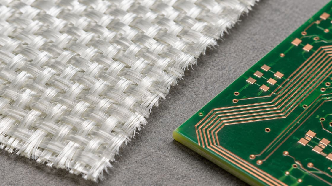
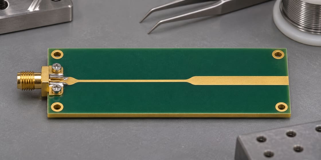
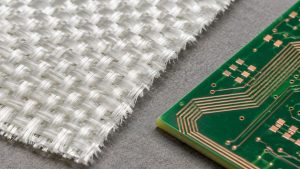
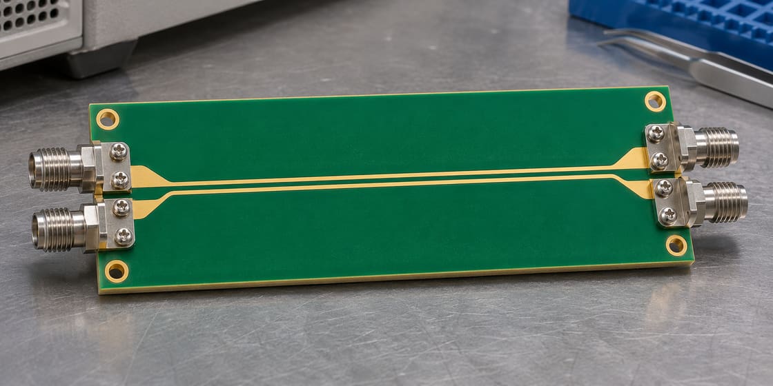
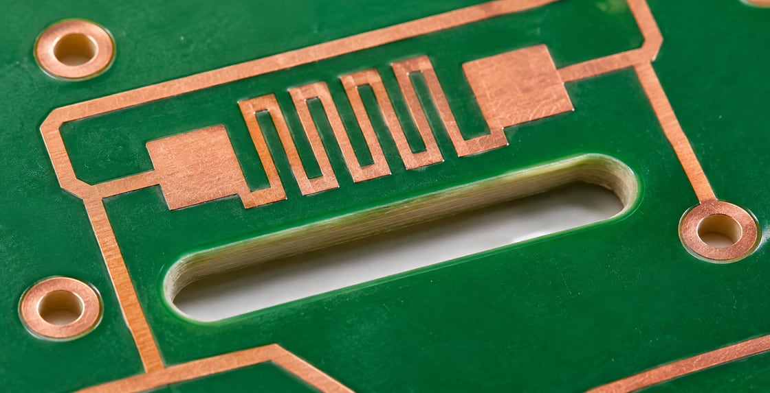
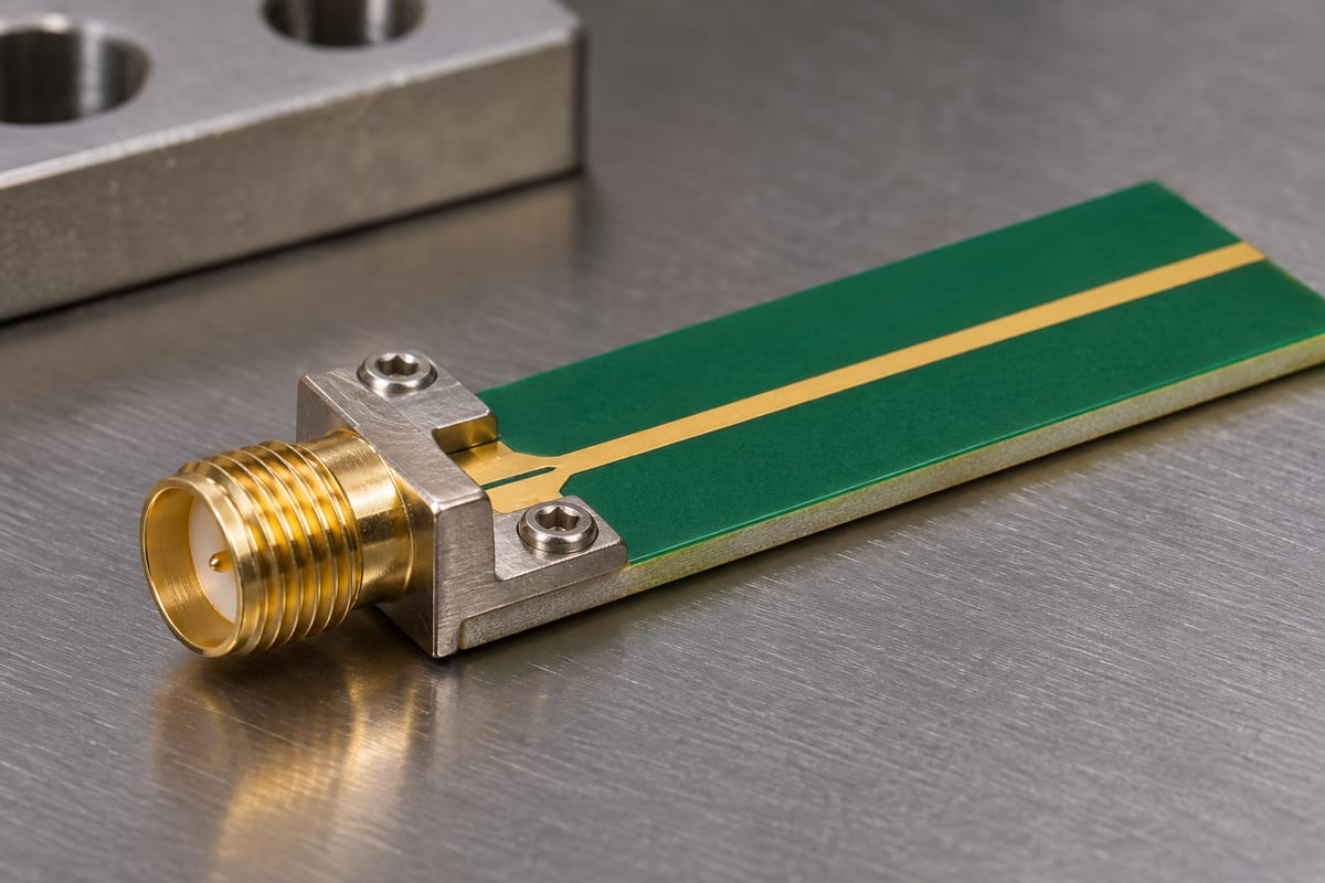
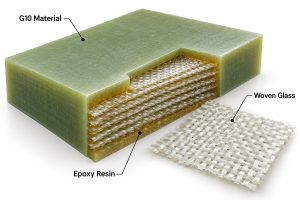
Woven glass reinforcement beside a PCB trace coupon
Woven glass reinforcement beside a PCB trace coupon. AI-generated illustration, not a measurement or production record.

This guide explains the mechanism, compares mitigation choices and shows how to include weave effects in a timing review. It focuses on differential-pair delay, not on changing a laminate merely because its published bulk dielectric constant is lower.

What creates glass weave skew?

A woven reinforcement has glass-rich yarn regions and more resin-rich spaces between them. A trace following one region for a long distance can experience a different effective dielectric environment from its partner. Effective permittivity is the combined field-dependent property seen by the transmission line, not simply the bulk value of one ingredient.

The effect depends on the material construction and how the traces align with it. A controlled-impedance stackup describes the nominal line, but small local differences can remain important when the available timing margin is narrow.

What parameters belong in the timing review?

Start with delay and margin at a defined reference plane. Geometric dimensions are inputs; arrival-time difference is the quantity the receiver ultimately sees.

Input Unit Purpose
Pair delay difference ps Compare with allowed budget
Coupled route length mm Identify long exposed regions
Copper length mismatch mm Separate geometry contribution
Glass construction Style and treatment Identify actual reinforcement
Route to weave angle Degrees Assess repeated alignment
Material variant Full construction Avoid generic FR-4 assumptions

Do not borrow a skew limit from an unrelated interface. Use the applicable device and link requirements, then allocate margin among the PCB, package, connector and other parts of the path.

Equal length vs equal electrical delay

Equal length removes one source of mismatch but not all of them. In a simplified uniform transmission line, delay per unit length scales approximately with the square root of effective permittivity. A different local effective value can therefore change travel time along two equally long routes.

That approximation is a teaching model. It does not predict a woven laminate’s exact local behavior, because real fields span several materials and the construction is not uniform along the path. Use it to understand why a ruler is not a complete timing instrument.

A worked example of the remaining margin

Suppose a hypothetical link allocates 8 ps to PCB pair mismatch. A simulation or representative measurement already attributes 3 ps to the routed geometry. Only 5 ps remains within that allocation for other PCB contributions under the chosen budgeting method.

You cannot conclude that the weave contribution is zero because the layout tool reports equal length. Also, do not add independent estimates without checking whether they describe the same effect twice. This example is budget arithmetic, not a universal interface limit.

Compare routing and material mitigation choices

Choose a method that addresses how both traces sample the reinforcement, then evaluate its effect on the rest of the layout.

Option Intended benefit Trade-off to verify
Route at an angle Cross multiple yarn regions Extra length and routing space
Rotate panel image Change trace-to-weave alignment Panel use and fabrication agreement
Use spread-glass construction More uniform local structure Exact material and stackup availability
Qualified weave-aware stackup Known construction and evidence Substitution control and cost

No option guarantees zero skew. The useful question is whether the chosen construction and geometry leave sufficient margin in the actual link.

Why route angle must be relative to the weave

An angle relative to the board edge matters only if the reinforcement orientation is known relative to that edge. A pair drawn diagonally can still align poorly with a rotated material. State the intended relationship in the fabrication discussion rather than relying on the appearance of the layout.

Texas Instruments’ high-speed layout guidance discusses routing and image-rotation approaches. Treat those examples as mitigation guidance; confirm the appropriate construction and geometry for your interface.
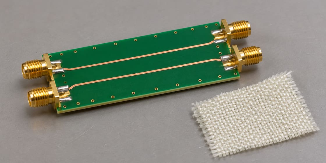
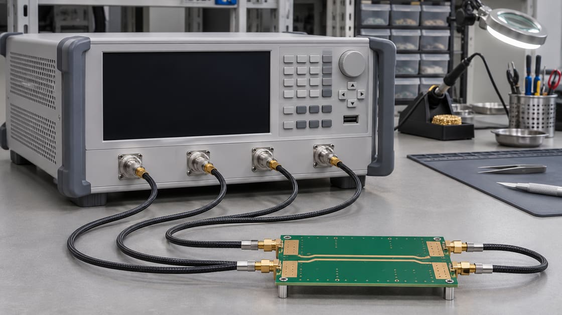
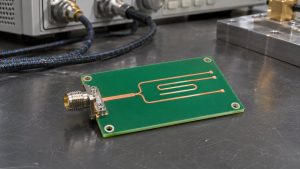
Differential trace coupon with coax connectors beside woven glass
Differential trace coupon with coax connectors beside woven glass. AI-generated illustration, not a measurement or production record.

What spread glass changes and what it does not

Spread-glass reinforcement distributes yarns more uniformly than an open, concentrated weave pattern. That can reduce local differences sampled by nearby traces. The designation must still identify a real supplied material construction; “spread glass” is not a complete stackup specification.

It does not remove connector asymmetry, via mismatch or an unsuitable return path. Keep each mechanism distinct during review so a material upgrade is not used to avoid correcting an ordinary layout problem.

Why nominal Dk is not a weave-skew specification

A data-sheet dielectric constant summarizes a material under a stated method and condition. It does not directly state how much two adjacent traces will differ over a particular route. Two constructions with similar nominal Dk can still distribute their reinforcement differently.

Ask for the actual glass styles, resin system and construction relevant to the routing layer. If the supplier proposes a substitute, compare that construction and its evidence rather than approving it solely on the nearest bulk Dk number.

Avoid fixing the wrong kind of mismatch

A connector launch, unequal via transitions or different reference conditions can create delay or mode-conversion problems that resemble a pair imbalance. Review those discontinuities before attributing a measured difference entirely to weave.

The BestPCBs SCD21 mode-conversion guide addresses a related measurement result. Mode conversion can be evidence of imbalance, but it does not identify glass weave as the cause on its own.

Use a coupon that represents the real routing

A useful comparison keeps the stackup, routing layer, geometry, length and reference method under control. Include the proposed orientation or construction change. Keep launch and fixture contributions consistent so their difference is not mistaken for a laminate improvement.

Sampling matters because trace placement relative to the weave can vary. A single favorable coupon is not proof that every route or panel position will behave identically. Agree the evaluation plan with the fabricator and signal-integrity team.

Keep the mitigation in the released fabrication package

Record the approved laminate construction and any agreed image rotation or orientation requirement. Make substitution review explicit. Otherwise, a repeat order can preserve the copper artwork but change the reinforcement arrangement behind the original timing evidence.

Separate a requested process from a verified outcome. A drawing note asking for a particular construction is not a measurement report. Retain both the material identity and the relevant coupon or link evidence with the design revision.

Decide whether the link actually needs a change

A weave-aware review is most useful when the route length, signaling requirements and remaining margin make the effect significant. Do not add routing complexity or an expensive material solely because the mechanism exists. Compare the proposed change against the timing budget and practical verification evidence.

For a Best Technology stackup review, send the interface requirements, layer construction, long pair routes and timing evidence to sales@bestpcbs.com. Ask for construction and orientation confirmation before releasing a material-dependent mitigation.

FAQ

Can glass weave matter when a pair is perfectly length matched?

Yes. Matching copper length addresses geometric mismatch, while local dielectric variation can change delay per unit length. The significance depends on the route and available timing margin. Keep both effects in the review and use representative construction evidence rather than assigning a universal skew value.

Is there a single maximum length below which weave never matters?

No universal cutoff applies to every interface and laminate. Sensitivity depends on route geometry, construction, alignment and the allowed delay difference. A short low-demand link may have ample margin, while a stricter design needs a quantified review. Use the actual budget rather than a general length rule.

Does routing at 45 degrees always solve the problem?

No. The relevant angle is relative to the reinforcement, not just the board outline, and the actual construction still matters. An angled route can help both traces sample different regions, but it also changes route length and space. Verify the resulting link rather than assuming a particular angle guarantees success.

Can I compensate weave skew with a fixed length adjustment?

Be cautious if the underlying local variation is not repeatable across builds. A fixed compensation can correct one measured specimen while worsening another. Distinguish deterministic geometry from material variation and confirm the behavior across the agreed sample set before applying a production adjustment.

Does lower Dk automatically mean lower weave skew?

No. Bulk permittivity and local uniformity are different properties. A material with a lower published Dk can still have a construction that creates unequal local environments for two traces. Compare the actual reinforcement and route conditions, and keep the test method attached to any numeric material data.

Can I infer glass weave from an impedance report alone?

Not reliably. An impedance report can show whether the measured line meets its stated target, but it does not isolate the cause of pair delay mismatch. Use suitable delay or mixed-mode measurements and a controlled comparison if the investigation needs to distinguish weave from launches or other asymmetry.

Should every high-speed board use spread glass?

No. Select it when the construction and link margin justify the change, and verify availability and substitution control. Other design factors may dominate the link. A stackup decision should balance electrical evidence, routing practicality and manufacturing repeatability rather than treating one reinforcement label as a blanket requirement.

Can a repeat order change skew without changing the artwork?

It can if the material construction, orientation or other relevant conditions change. Even with a controlled construction, local alignment can vary. Preserve the approved stackup and process agreements, review substitutions, and use an appropriate sampling plan when timing performance depends strongly on reinforcement behavior.
You may also like

PCB TDR Fault Distance: Convert Round-Trip Time
Friday, November 6th, 2026

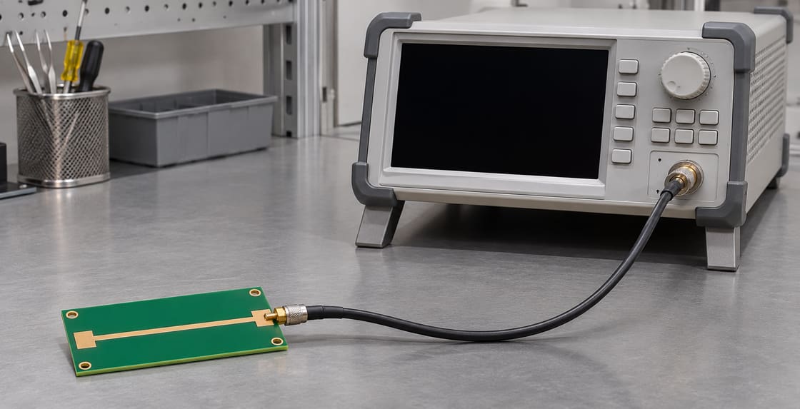
On a PCB TDR reflection trace, the pulse travels to a discontinuity and back. For a uniform section, one-way distance equals propagation velocity times round-trip time divided by two. Check whether the instrument already displays one-way distance before applying the conversion, then map the result to the actual route rather than measuring across the board.

PCB transmission-line coupon connected to a test instrument
PCB transmission-line coupon connected to a test instrument. AI-generated illustration, not a measurement or production record.

Why the reflection takes a round trip

Time-domain reflectometry launches a fast change and observes the return at the measurement side. A mismatch can reflect part of that signal. The time difference from a defined reference to the reflection includes travel in both directions.

What to record with a marker

A distance is only as useful as its reference and velocity model.

Field Unit or definition Example only
Time interval ns, measured as round trip 0.80
Propagation velocity mm/ns 160
Reference plane Physical boundary Coupon input launch
Computed one-way distance mm 64
Instrument axis Time or configured distance Confirm before converting

Convert the sample reflection time

Multiply 0.80 ns by 160 mm/ns and divide by two to get 64 mm. Without the divisor you would look near 128 mm. Keysight’s TDR concepts describe round-trip reflection timing and calibration with a known line.

TDR time vs displayed distance vs TDT

First identify what the instrument marker actually reports.

Reading Meaning Conversion
Raw reflection interval Outbound and return time Multiply by velocity and divide by two
Configured TDR distance Instrument-scaled distance Verify settings; do not halve again
Through transmission delay One-way delay for a defined transmission measurement Do not use the reflection divisor

Calibrate velocity on a known route

Use a known physical length with the same relevant transmission geometry when practical. If a 40 mm reference span corresponds to 0.50 ns round trip, its inferred velocity is 160 mm/ns. Use the same reference convention when applying that value to the unknown feature.

Set the reference before interpreting the event

Decide whether your origin is the instrument port, the connector plane or the PCB trace start. The cable and launch contribute delay if they remain in the measurement. Record the calibration or fixture treatment rather than quietly assuming time zero is at the board.

PCB test coupon with a coax launch and a trace transition
PCB test coupon with a coax launch and a trace transition. AI-generated illustration, not a measurement or production record.

Map distance along the route

Use cumulative distance along the traced conductor. A via or a bend can make straight-line separation misleading. Note which layer and routing segment the candidate feature occupies and check the positions of known launch or termination events.

Use separate delays for mixed structures

A cable, microstrip and stripline need not share one velocity. Account for their segment delays or use a suitable calibrated reference. Applying a single factor to an entire mixed route may move the apparent feature even when the reflection time is correct.

Know how close two events can be

Finite effective rise time and bandwidth can make neighboring reflections overlap. An apparent peak may represent more than one feature. Do not infer a precise physical location from a cursor whose resolution exceeds the information in the measurement.

Check alternatives before naming the fault

An impedance change, connector transition, stub or termination can all create a reflection. Compare a good unit or controlled fixture and use the layout to narrow possibilities. The marker alone does not tell you whether the feature is an open, a defect or a normal transition.

Keep impedance and location separate

The reflection magnitude and inferred impedance describe the event under the test conditions. Its delay estimates where to look. Compare with the BestPCBs signal transmission guide for other channel verification tasks.

Save the setup with the result

Preserve raw data, axis settings, velocity basis, reference plane, route coordinates and candidate features. For a stackup or test coupon manufacturing review, share the files with Best Technology at sales@bestpcbs.com.

FAQ

Why is my calculated distance twice the expected value?

The marker may be showing round-trip time, and the calculation may have omitted the divisor of two. Confirm the axis and reference before changing the velocity setting. If the display is already calibrated in one-way distance, do not apply the divisor again.

Can I use the speed of light for a PCB trace?

Not as the actual line velocity unless the propagation medium and geometry support it. A PCB transmission line normally propagates more slowly. Use a measured or modeled velocity appropriate to the actual route, and label any screening assumption in the test record.

Can I use the same velocity factor on every layer?

Not without checking the construction. Different layers can have different dielectric materials, field distributions and reference structures. If the route crosses layers, evaluate each relevant segment or compare with a calibrated structure that represents the full path under the same conditions.

Is the distance the same as straight-line distance on the board?

No. It corresponds to travel along the electrical path. A serpentine can place a feature far along the route while it is physically close to the connector in a top view. Map against cumulative trace distance, including relevant transitions, instead of a ruler across the board.

Can a known cable remove all fixture effects?

A known cable can help establish timing, but launches and adapters can still contribute reflections or delay. Set the correct calibration reference and inspect a suitable reference fixture. Do not assume velocity calibration is equivalent to removing fixture mismatch or loss.

Why does a strong reflection not prove a broken trace?

A normal connector, impedance step or termination can also produce a strong return. Compare with the expected layout and a known good reference. Use additional evidence before assigning the reflection to a crack, open or manufacturing defect at the estimated location.

What if the instrument shows distance in free space?

Confirm whether the plotted axis already applies the medium velocity factor. A free-space-scaled distance is not the physical PCB distance. Follow the instrument documentation and verify with a known length before accepting a marker position as a measured route location.

Can I use the same formula for transmission delay?

Only after identifying the timing convention. Transmission from one end to the other is ordinarily a one-way measurement, so its distance relation lacks the reflection divisor. Keep the acquisition mode and reference planes in the report so the calculation is not misapplied.

You may also like

SCD21 on a PCB: Find Differential-to-Common Conversion
Friday, November 6th, 2026

SCD21 measures how much of a differential stimulus at logical port 1 emerges as common mode at logical port 2. On a PCB pair, skew, unequal losses or unequal transitions can contribute. First confirm the port mapping and fixture response; otherwise the test setup can look like a layout problem.

Differential PCB test coupon with coaxial launches
Differential PCB test coupon with coaxial launches. AI-generated illustration, not a measurement or production record.

How to read the letters and port numbers

The output mode comes first and the input mode second: C is common, D is differential. The 21 identifies output at logical port 2 with stimulus at logical port 1. Keysight’s balanced-measurement reference explains this convention.

What to capture with a plot

Record the data needed to repeat the comparison.

Parameter Unit or definition Check
Sweep Hz and points Same band and frequency grid
Logical port mapping Two conductors per end, with polarity Matches the physical fixture and file order
Reference impedances Ω, including normalization Same convention for compared traces
Calibration planes Physical locations Same fixture inclusion or removal
Reported response dB versus frequency Compare the correct term and direction

SCD21 vs SDD21 vs SDC21

These terms describe different input and output modes.

Term Input and output What it tells you
SCD21 Differential in, common out Forward differential-to-common conversion
SDD21 Differential in, differential out Forward differential transmission
SDC21 Common in, differential out Forward common-to-differential conversion

Use a skew example as a diagnostic clue

In an ideal equal-loss, uncoupled pair with otherwise identical matched paths, delay mismatch alone produces a converted magnitude of |sin(πfΔt)| relative to the incident normalized differential wave for lossless paths. At 5 GHz and 5 ps, this is about 0.0785, or −22.1 dB. This is a simplified example, not a channel acceptance limit or a way to infer skew from every measured trace.

Check unequal amplitude as well as delay

If the two paths deliver different amplitudes, they do not cancel perfectly in the common-mode sum even with equal delay. Compare individual path responses before adding length. Equal drawn trace length cannot fix a connector or launch that attenuates one conductor more.

Verify the physical port map first

Map the two conductors at each end to the analyzer’s logical pairs. A swapped port or polarity can alter the interpretation of a mixed-mode plot. Preserve the port map with the raw single-ended S-parameter file so the conversion can be repeated.

Network analyzer and a PCB coupon on a test bench
Network analyzer and a PCB coupon on a test bench. AI-generated illustration, not a measurement or production record.

Establish the fixture baseline

Compare a known balanced reference or verification coupon with the DUT. Verify repeatability and the calibration planes before attributing a conversion peak to the board. For related measurement boundaries, see the PCB fixture de-embedding guide.

Inspect asymmetry where the pair changes geometry

Compare both launches, vias, reference transitions and termination areas. For example, one conductor may encounter a different pad or return path near a layer change. Check the structure at the same point on both sides instead of assuming the straight runs are the only source.

Interpret broad trends and narrow peaks differently

A gradual increase can be consistent with simple delay mismatch over a limited band. A narrow peak may suggest a discontinuity, resonance or fixture effect. Neither shape alone identifies root cause. Compare changes between controlled layout or fixture variants.

Keep conversion and emissions evidence separate

Converted common mode can be relevant to emissions, but a conversion plot does not establish regulatory pass or fail. Coupling to cables, enclosure features and the operating stimulus also matter. Verify at the appropriate system level when emissions are the concern.

Use the product’s requirement, not a generic threshold

Set the allowable conversion over the specified band and reference planes using the actual system or interface requirement. Do not apply a rule from a different connector or application. Document the noise floor or repeatability limits near the acceptance boundary.

Deliver a reproducible comparison

Save the port map, stackup, fixture setup, raw data, conversion convention and limits with the plots. For a PCB or coupon manufacturing review, share those requirements with Best Technology at sales@bestpcbs.com.

FAQ

Does more-negative SCD21 usually mean less conversion?

Yes when comparing magnitude in dB under the same normalization and reference planes. A more-negative number represents a smaller converted wave relative to the input. Ensure the measured response is above the useful noise floor before drawing conclusions from small differences.

Can good insertion loss hide conversion?

A channel may have acceptable differential transmission and still generate common mode. Plot SDD21 and SCD21 as separate quantities across the same band. Check each against the appropriate requirement rather than relying on a single loss trace to characterize every response.

Can I read SCD21 from a single-ended two-port measurement?

Not from one ordinary two-port trace alone. The conversion depends on the responses of both conductors in each logical port under the applicable normalization. Use suitable multiport measurement data and record the port pairing and calculation convention used for the mixed-mode result.

Does zero skew guarantee zero mode conversion?

No. It removes one possible mechanism but does not eliminate amplitude imbalance or asymmetry in launches, return paths and terminations. Check the complete channel and fixture. Equal timing in one part of the path cannot establish balance at every discontinuity or frequency.

Can I use SCD21 to locate a fault by itself?

It can show where in frequency the conversion is observed, but not automatically where on the board it originates. Combine it with reference structures, controlled layout changes or suitable time-domain analysis. Verify the fixture before attributing the result to a specific feature.

Should I compare two plots with different reference planes?

Not as if they represent the same DUT. One may include a connector or launch that the other removes. Align the planes or explicitly describe the difference. Preserve the raw measurements so another engineer can reproduce the comparison under the intended convention.

Can a software port swap repair a real board problem?

It can correct a bookkeeping error if the measured ports were paired incorrectly, but it cannot change a real electromagnetic imbalance. Verify the physical assignment before reprocessing the data. If the conversion remains, check the fixture and compare equivalent features of both conductors.

Is there a universal pass limit for SCD21?

No. The acceptable magnitude depends on the interface, band and system requirement. Set the limit with defined reference planes and test conditions, and account for fixture repeatability. Do not transfer a limit from an unrelated assembly just because the two channels use similar impedance.

You may also like

Differential Via Antipads: Shared Oval or Separate?
Friday, November 6th, 2026

A shared oval antipad can reduce local capacitance in a differential via transition, but it also removes plane copper. Compare it with two separate openings in the actual stackup. Keep the signal pair, return vias and fabrication clearances in the model rather than enlarging the cutout by itself.

What an Antipad Does

An antipad is a clearance in copper around a feature that must not connect to that copper. At a signal via, it also changes the electrical coupling between the via and the reference plane. Texas Instruments’ differential via article discusses those effects and a shared oval example.

High-speed PCB with closely spaced via features
AI-generated illustration, not a view of a hidden antipad.

Why Two Openings Are Not the Same as One

Two separate clearances can leave a copper bridge between them. A shared opening removes that bridge and changes the field around both vias. Neither arrangement is universally better; compare the transition and surrounding reference structure.

Detailed Model Inputs

Input Unit or record Purpose
Via pitch mm Sets pair spacing
Pad and barrel Finished geometry Defines the conductor
Opening by layer Shape and dimensions Describes plane clearance
Return vias Position and reference net Represents the return path
Stub and layer pair Length and layer IDs Describes the transition

Shared Oval vs Separate Antipads

Feature Separate openings Shared opening
Plane between the vias May retain copper Removed in the shared region
Electrical review Coupling with retained bridge Coupling with common opening
Fabrication review Width and stability of copper web Clearance to nearby features

Worked Example: Check Whether a Web Remains

For two aligned circular openings of 0.45 mm diameter with centres 0.55 mm apart, their nominal edge separation is 0.10 mm. That is only the artwork value for this hypothetical case. Verify the intended finished web and tolerance or compare a shared opening instead.

Keep Both Sides of the Pair Comparable

Review symmetry around each via, the nearby reference connections and any asymmetry introduced by other routing. An electrically asymmetric environment can affect the differential transition. Do not judge the pair only by whether its two hole sizes match.

Do Not Remove Return Copper Without Checking the Path

A larger opening can clear copper around the signal vias but also reshape the nearby reference region. Review where return current can transfer between planes. If a neighbouring path becomes narrow or interrupted, assess that change as part of the same comparison.

Model the Stub and Pads With the Opening

The pad, barrel, stub and antipad contribute to one transition. A short local impedance change is not automatically attributable to the opening. Keep the geometry consistent between alternatives and use an appropriate model when the bandwidth or loss budget makes the distinction important.

Review Layer-Specific Clearance

The same opening is not necessarily appropriate on every layer. Check plane assignments, copper features and any controlled-depth operation. For the broader treatment of unused barrel, see the BestPCBs via stub guide.

Compare an Actual Test Structure

For a sensitive link, use a structure that reproduces the layer change, openings, nearby grounds and routing. A straight impedance coupon alone cannot demonstrate the transition. Agree on the test objective and how fixture effects will be interpreted.

PCB coupons near coaxial fixtures on a lab bench
AI-generated illustration of test context, not measured evidence.

Keep the Fabricator’s Clearance Rules Separate

The model answers an electrical question; the fabricator confirms which openings and copper features can be built. Check the artwork, layer-by-layer clearances and applicable tolerances. If the final geometry changes, rerun the relevant comparison before accepting the build.

Record the Selected Geometry and Evidence

Keep the via dimensions, opening shape, layer map, return arrangement and verification result together. Record why the selected option met the actual requirements. If the stackup changes, revisit the transition instead of assuming an old clearance is still appropriate.

Discuss a High-Speed Stackup

Share the layer pair and via geometry with Best Technology.

FAQ

Is a shared oval antipad always better?

No. A shared opening changes capacitance and also removes plane copper between the vias. The right choice depends on the stackup, return paths, dimensions and electrical target. Compare both options and verify the fabrication constraints instead of adopting the oval solely because a reference design used it.

What if two separate openings overlap?

Then they no longer preserve a complete web between them in the overlapping area. Review the actual resulting shape rather than treating the artwork as two independent circles. Confirm the intended clearance with the fabricator and use the correct merged geometry in any electrical model.

Is the antipad the same as the via pad?

No. The via pad is a conductor intended to connect at an applicable layer. The antipad is an opening in surrounding copper where a connection is not intended. Identify both on the relevant layer so their sizes and purposes are not accidentally swapped.

Can I enlarge the antipad to fix any impedance dip?

Not reliably. A dip can involve multiple parts of the transition, and changing the opening may affect return geometry or nearby features. Compare the suspected mechanism with a suitable model or measurement before changing the layout, and check the impact on the rest of the path.

Do return vias still matter for a differential pair?

Yes, evaluate them as part of the actual reference transition. Differential signals interact with nearby copper, and asymmetry or a reference change can matter. Confirm where the references connect and model the geometry that will be built rather than assuming the pair needs no return review.

Will a standard impedance coupon show the effect?

Only if the coupon includes a representative transition and the method can resolve it. A straight uniform trace checks a different structure. If the antipad decision is important, specify the relevant layer change and geometry and agree how the result will be interpreted.

Can different layers use different antipad shapes?

They can be designed differently when the electrical and manufacturing requirements support it. Check the relevant plane, clearance and nearby geometry on each layer. Document the actual shapes for the model and fabrication release rather than relying on a single label for the entire via.

What should I send for a transition review?

Send the stackup, via pitch, pad and barrel dimensions, layer-specific openings, return-via positions and stub details. Include the interface requirements and intended measurement or simulation scope. Those inputs let the reviewer assess the transition without guessing what the clearance drawing means.

You may also like

PCB Return Path Guide: When a Trace Crosses a Slot
Friday, November 6th, 2026

A trace can look continuous in CAD while the copper that carries its return current is interrupted. If a fast signal crosses a gap in its reference plane, first look for a route over continuous copper. A return bridge is not a default fix, especially if the gap provides safety isolation.

What Current Is Returning?

A driver and receiver are part of a current loop. At high frequencies, nearby reference copper helps provide a low-inductance return path. Trace length alone describes only the outward part of the loop. The Texas Instruments high-speed layout guide discusses how reference-plane gaps interrupt that path.

Bare PCB with a routed slot and visible copper pattern
AI-generated illustration of a physical slot; not evidence of an internal reference plane.

A Physical Slot Is Not the Only Interruption

A milled opening removes board material. A copper void removes reference metal without necessarily cutting the substrate. A row of overlapping antipads can also interrupt copper. Inspect the actual reference layer rather than assuming that only visible board cutouts matter.

Detailed Layout Parameters to Record

Input Unit or record Why it matters
— — —
Signal and reference layers Layer IDs Identifies the intended return
Void location and width X/Y and mm Locates the interruption
Trace-to-reference spacing mm Helps evaluate field coupling
Edge rate Time and definition Informs relevant frequency content
Reference connection Net, via and location Defines the intended return transfer

Reroute vs Change Layers vs Bridge

Option Use when Verify
— — —
Reroute on the same layer Continuous reference exists nearby Entire new path and timing
Change signal layers New reference is viable Return transfer and via geometry
Approved AC bridge Circuit permits the two regions to couple Component parasitics and actual response

Trace the Reference From Source to Receiver

Overlay the signal and its reference copper. Follow each segment, bend and transition. Name the reference after each layer change; the same net name on two layers does not identify the physical path between them. Use the BestPCBs ground-plane guide for the wider layout review.

Worked Example: A Clock Crossing a Connector Void

Suppose a clock trace on L1 references L2 but crosses a copper keepout under a connector. One revision adds 8 mm of trace to route around the void over continuous L2. Compare its timing and signal integrity with the short crossing. The added length is an example, not a rule that longer routing always wins.

Check a Differential Pair as a Real Pair

A differential pair still interacts with reference copper. Geometry changes or imbalance can disturb the pair and contribute to mode conversion. Review both traces and the corresponding plane region. Do not assume that a pair is exempt just because its signals are complementary.

A Stitching Via Cannot Bridge Every Gap

A nearby return via can help connect same-net reference planes at a layer transition. It cannot connect two regions unless there is a legitimate conductive path between them. Confirm the net and layer connections before adding a via that looks useful only in plan view.

Keep Intentional Isolation Intact

Do not bridge a safety or functional isolation gap as a layout cleanup. An inter-domain signal may require an isolator or another approved architecture. Treat any proposed change across the barrier as a separate engineering decision with its applicable clearances and requirements.

Look for a Discontinuity in the Right Test

An impedance plot can help locate a reflection, while eye or emissions testing addresses different system outcomes. Where possible, compare two otherwise similar layouts to see what the routing change does. A standard coupon that lacks the gap will not validate that local crossing.

High-speed PCB and oscilloscope on an electronics test bench
AI-generated illustration of a test environment, not a measured result.

Recheck the Manufacturing Output

A plane shape can change after copper repour, keepout edits or layer export. Review the released copper artwork with the routed signal, especially at connector pin fields and plane boundaries. Record the layer pair, affected net and evidence for any accepted exception.

Decide What to Change First

Start by restoring a continuous reference without touching isolation or power architecture. If that is not possible, compare an alternate layer and an approved reference transfer. Use the interface’s performance targets to decide whether further simulation or hardware validation is warranted.

Request a Stackup Review

Share the affected layer pair, connector layout and net requirements with Best Technology.

FAQ

Is a trace over a small gap always a problem?

The impact depends on the gap geometry, trace-to-plane spacing, edge rate and the return paths available nearby. Do not assume the effect is negligible because the gap looks small at board scale. Compare the actual stackup and verify the relevant channel or emissions requirement if necessary.

Is clock frequency the same as edge rate?

No. Frequency describes how often the clock repeats, while edge rate describes how quickly it changes level. A low repetition-rate signal can still have fast edges. Review the driver’s transition behaviour and interconnect geometry when deciding whether the crossing needs high-frequency attention.

Can a capacitor fix every plane split?

No. A capacitor may provide an AC path in a design that permits it, but connection inductance, placement, frequency and safety constraints matter. Do not use it to bypass an isolation requirement. Prefer a route over continuous reference copper when it meets the design goals.

Do I need a ground via every time the signal changes layers?

Review whether the signal’s reference changes and where the corresponding return current can transfer. A nearby same-net connection can be useful when two reference planes are involved. A via is not a substitute for identifying the reference layers, and unrelated reference nets must not be shorted.

Can I route around the slot if the trace gets longer?

Often that is a useful option to compare, but validate both delay and routing constraints. Estimate the additional path length, check pair matching or timing where relevant, and review the entire return path. Do not judge either option on trace length alone.

Does a ground pour on the trace layer fix the issue?

Only if the resulting geometry and connections provide a suitable reference for that specific route. Isolated or weakly connected copper is not automatically a good return path. Check the copper spacing, grounding and stackup, and use an appropriate model when the behaviour is important.

Will an impedance coupon show a slot crossing?

Only if it intentionally represents the relevant structure. A straight coupon on uninterrupted reference copper can characterize the ordinary trace but not a local return interruption under a connector. Check what the coupon represents and use a targeted structure or board measurement if the crossing must be validated.

Should I merge two separate grounds to avoid the gap?

Do not merge domains simply to make a routing overlay look cleaner. First establish why they are separated and what signal must cross. Follow the system’s safety and circuit requirements, and consider rerouting or an approved interface architecture before modifying the intended isolation boundary.

You may also like

DDR Fly-By Topology Guide: Routing and Write Leveling
Friday, November 6th, 2026

In a DDR fly-by topology, shared signals such as clock, address and command travel along a route that passes the memory devices in order. The clock therefore reaches each device at a different time. Where supported, write leveling compensates for the clock-to-write-strobe timing difference at each device; it cannot repair a poorly terminated or incorrectly routed signal.

Consider a hypothetical single-rank board with two discrete DDR3 devices. A controller drives the shared clock and command network, and each device has its own data byte lanes in this example. The goal is to review the route and collect evidence before debugging firmware or changing the board.

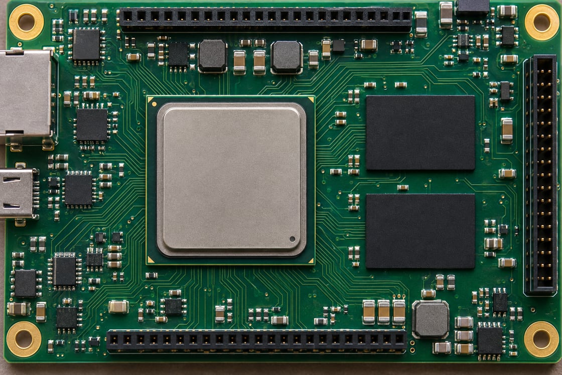
Embedded processor board with two rectangular memory packages
AI-generated illustration of a processor and adjacent memory packages, not a reference layout.

Follow the Clock Past Both Memory Devices

Think of the shared route as one road with two stops. The first receiver sees the edge earlier because its route from the controller is shorter in time. The second sees it later. The receivers do not regenerate the clock for the next device; the PCB interconnect carries it past both loads.

Fly-By vs Balanced T vs Point-to-Point

These topologies distribute a signal in different ways, and the controller documentation determines which is allowed for a particular group. Matching all loads to the same delay is not automatically the design goal on a fly-by net.

Topology Routing shape Key check
Fly-by Receivers along a shared route Local timing at each load and far-end treatment
Balanced T Branches arranged for similar delays Branch matching and reflections at the junction
Point-to-point One route between two endpoints Endpoint timing and reference continuity

Map Each Signal Group Before Routing

Make a routing table from the controller and memory documentation. For this example, CK means the clock pair, CA refers to command and address, DQ carries data, and DQS is the strobe used to time the data. Check control signals separately instead of assuming that every non-data pin belongs on one shared route.

Build a Timing Budget in Picoseconds

Use delays at the receiver pins rather than simply comparing whole-net lengths. The following values are invented to demonstrate the calculation, not electrical limits. A board-specific budget must include the applicable controller and DRAM rules, package delays where required, and actual routing geometry.

Illustrative parameter Device A Device B
CK path delay 180 ps 330 ps
Write DQS path delay 200 ps 220 ps
DQS minus CK path delay +20 ps −110 ps
Relative difference between locations Baseline 130 ps earlier relative to local CK

The example assumes simultaneous launch for the arithmetic only. It does not calculate the real phase at the receiver, a training register value, or compliance margin.

Match Shared Signals at Each Receiver

Check the controller-to-A segment and the controller-to-B segment separately using the constraints for the signal group. A report that ends at the last termination can hide mismatches at A. Export a source-to-load delay report with named endpoints and verify which trace and via segments are included.

Keep Data Lane Checks Separate From Fly-By Checks

In this single-rank example each data lane is reviewed against its own strobe. Do not route DQ along the address chain or assume that a length match between two different byte lanes proves that either lane is valid. Use the lane mapping and timing constraints for the actual controller.

Place Termination for the Route You Actually Built

Follow the device-specific termination scheme and place the far-end elements where the approved topology calls for them. A resistor footprint is not enough: review the stub from the main route, the return path and the termination rail where applicable. Clock and single-ended command signals may require different termination arrangements.

Memory packages and small passive components on an embedded board
AI-generated illustration of memory packages and nearby passives; placement and values are not design instructions.

Check the Return Path Through Layer Changes

Check every reference transition as well as trace length. A via or plane gap can change the return-current path and create a discontinuity that the length report does not show. Review layers and references with the approved stackup before tuning; then evaluate the resulting interconnect with the tools and models specified for the interface.

What Write Leveling Changes

Write leveling adjusts the timing of the write strobe relative to the clock observed by the receiving memory. In the AMD PG150 example, the controller drives DQS and the memory returns feedback on DQ during calibration. The output is a controller timing adjustment, not a change to the PCB routing.

What Write Leveling Cannot Fix

Training is not a cure for invalid pin mapping, a missing reference path, a noncompliant termination, or excessive distortion. If the required correction is outside what the specific controller can train, a board can also fail despite having the intended topology. Check supported settings and ranges before interpreting a failure as a layout defect.

Use Failure Patterns to Narrow the First Debug Step

Start with the failing lane or rank, not a new board revision. A failure isolated to one byte lane suggests checking that lane’s mapping, strobe and assembly first; a shared failure across devices also warrants reviewing clock, reset, power and configuration. These are starting points, not proven causes. Save the training logs and compare with the released design.

Release With Routing and Bring-Up Evidence

Keep the routing constraints, per-load delay report, approved stackup, topology and termination notes together. Then record the hardware and firmware revisions used for bring-up and run the approved memory validation at the intended operating conditions. A successful boot is useful evidence, but it does not prove timing margin across the product’s operating range.

FAQ

Can both devices have the same full trace length?

That is not the normal objective for a clock that passes the devices sequentially. Focus on the required local relationship at each receiver and on the controller’s allowable path delays. Adding length just to equalize unrelated endpoints can introduce geometry and delay that the routing guide never requested.

How do I measure only the first section of a fly-by net?

Define the controller and first receiver as the endpoints in a tool that supports source-to-load or pin-pair reporting. Then compare the reported path against the actual route. If the tool reports only total net length, extract the relevant segments explicitly rather than tuning against the length to the terminator.

Does a far-end resistor go on every signal?

No. Use the termination scheme required by the controller, memory and topology. The clock pair, shared single-ended signals, and data lanes can use different arrangements. Read the schematic and layout sections together because placement, connection and electrical value can all affect how a termination works.

Does write leveling replace read training?

No. They address different signal directions and timing relationships. The exact calibration sequence depends on the controller and memory. If the system passes one stage but fails another, record the actual failing stage before deciding which signals to inspect or which configuration to change.

Does a single DRAM device always need fly-by routing?

No multi-device chain is present when there is only one load on that particular net. However, use the approved topology and termination for the selected controller, device and rank arrangement. The number of packages by itself does not define the number of electrical loads on every signal.

Can I copy DDR3 constraints to a DDR4 board?

Do not copy them as a set. A similar topology name does not establish equivalent pin assignments, electrical requirements or allowable timing. Start from the target controller’s documentation for the exact memory interface, then check the memory data sheet and the proposed stackup before importing constraints.

Can a fabricated impedance coupon prove the memory interface works?

No. A coupon can provide evidence about the specified transmission-line construction under its test conditions. It does not measure the assembled receiver timing, lane mapping, connector behavior, or training range. Use it alongside the design review and assembled-board validation, not instead of them.

What does it mean when a board passes once but fails on a cold boot?

It shows an intermittent or condition-dependent symptom, not the root cause. Save the actual test conditions and failing training stage. Compare repeatable cold and warm runs with approved instrumentation and configuration, then investigate candidate issues such as timing margin, rail startup, or assembly rather than discarding the failing log.

References

AMD UG586: DDR3 component routing; AMD PG150: write leveling calibration. For related stackup questions see the Best Technology microstrip PCB guide.

Prepare a Stackup and Routing Review

Send the target interface, routing layers, controlled impedance requirements, and layout revision to sales@bestpcbs.com for a project-specific review request.

You may also like

PCB Fixture De-Embedding: Is the Loss in the Trace?
Friday, November 6th, 2026

A lab measures a PCB trace through two coax launches. The displayed result includes whatever lies between the measurement reference planes, not necessarily the trace alone. De-embedding estimates the response of the trace by removing a characterized fixture model. If the model does not match the real fixture, the corrected curve can be misleading.

Two PCB coupons beside a lab instrument
AI-generated illustration. The screen traces are fictional and do not show measured PCB loss or de-embedding results.

Start with one question: what is the device under test?

Suppose you want the loss of a straight trace on a radio board, excluding both connector launches. Call that trace the device under test, or DUT. If you instead want the loss of the assembled connector-to-connector board, the launches are part of the DUT. Both measurements are valid when clearly labeled.

What a reference plane means

A reference plane is the electrical boundary at which the measurement is defined. In this example, cable-end calibration may leave the launch and short lead-in traces inside the reported measurement. Mark the desired boundaries on the coupon drawing before interpreting a plot.

Calibration versus fixture removal

Calibration addresses the measuring system at the chosen planes. Fixture removal uses a model of the physical structure between those planes and the desired DUT boundaries. These operations are related but not interchangeable. Record both the calibration and fixture treatment used.

Why subtracting one number is not a general fix

A launch can reflect energy, so multiple reflections can affect the measured response. Adding or subtracting a fixed loss number does not generally remove those interactions. Use a model appropriate to the port arrangement and band, not a single correction guessed from a datasheet.

How a 2x Thru coupon helps

A 2x Thru joins representative fixture sections without the intended DUT. Measuring it gives an appropriate extraction method information about the fixture halves. In the radio-board example, the left and right launches on that reference structure must represent the corresponding launches in the DUT measurement.

Detailed measurement parameters to record

For an illustrative two-port job, document the intended sweep, for example 1–6 GHz, the reference impedance, for example 50 Ω, and the direction defined as port 1 to port 2. These are teaching inputs, not a universal requirement or measured result. S21 describes forward transmission under its stated reference conditions; display convention matters when comparing negative transmission in dB with positive insertion loss.

Measurement boundary What the result includes
Cable ends The launches and board path between the cable ends.
Trace ends The intended trace response after valid calibration or fixture treatment.
PCB fixture illustration 2
AI-generated physical illustration; not a company sample or a measurement record.

Choose between raw data, a model and calibration standards

Keep raw connector-to-connector data when those connectors are part of the product. Use a validated fixture model if you need the trace alone. A suitable calibration structure can instead set planes closer to the DUT. Which approach works depends on what standards or fixture structures can actually be made and characterized.

Make the reference coupon representative

Review stackup, launches, connector footprint, routing and local ground connections. A shorter trace on different material is not automatically a matching fixture. Keep the drawing revision and the as-built differences with the test record.

Check port numbering and fixture direction

Left and right fixture files may not be interchangeable. Confirm where each file starts and ends and whether its port order matches the instrument workflow. When the curve looks implausible, check this mapping before changing the board design.

Input Illustrative setting, not a limit
Frequency range 1–6 GHz in the example test plan.
Reference impedance 50 Ω in the example.
Forward direction Port 1 to port 2; report as S21 with the chosen display convention.
PCB fixture illustration 3
AI-generated physical illustration; not a company sample or a measurement record.

Recognize a correction that cannot be trusted

Unexpected apparent gain on a passive trace or a sharp feature not present in repeat tests warrants investigation. Check calibration, connection repeatability, fixture bandwidth and model quality. Do not treat a smooth curve alone as evidence that the correction is sound.

Compare measurements at identical boundaries

When comparing to simulation, define the same electrical length and reference planes. A model ending at the trace boundaries will not match a measurement that still includes the launches. Save both raw and corrected files so another engineer can see exactly what changed.

Release the test plan with the PCB

Include the DUT and reference coupon geometry, intended band, calibration setup, port mapping, model limits and acceptance basis. If the fixture is not representative, keep the result labeled as a combined measurement until the missing evidence is resolved.

FAQ

Should I always remove the connectors from the result?

No. If your deliverable is a complete connector-to-connector assembly, the launches may belong in the device under test. If the question is trace loss alone, define trace-end reference planes instead. Label the result so it is not compared with a measurement made at different boundaries.

Is a 2x Thru simply the DUT trace cut in half?

No. Its purpose is to represent the fixture sections joined without the intended device under test. How it is constructed and interpreted depends on the extraction method. Match the launches and interfaces to those on the DUT coupon, and document assumptions rather than relying on the name alone.

Can I reuse fixture files from another board revision?

Only after showing that the revised geometry and measurement setup still match the characterized fixture sufficiently for the task. A moved connector, different stackup or changed launch may alter the response. Retain the fixture file revision with the raw data so the comparison can be repeated.

Why can a passive trace appear to have gain?

A correction can amplify errors when the fixture model, measurement band or port mapping is unsuitable. Investigate the setup and repeatability rather than assuming the trace provides power gain. Compare the raw data and the characterized fixture before applying the corrected result to a release decision.

Does cable-end calibration remove a board launch?

Not by itself if the launch lies inside the calibrated measurement boundaries. Decide whether that launch is part of the reported device or needs a suitable fixture treatment. Record where the planes are set; calibration at the cable ends does not establish that the reported curve is trace-only.

Can I compare the corrected curve directly with any simulation?

Only after checking that simulation and measurement use matching reference planes, geometry, port direction and reference conditions. A trace-length or launch mismatch can produce differences unrelated to material quality. Keep both raw and processed measurements to make the comparison and its limitations transparent.

Can I use just a single loss number for the fixture?

A fixed correction may omit reflections, phase and variation with frequency. It is not a general replacement for a characterized fixture model. If a simplified method is used, state its assumptions and scope, and verify that it is adequate for the decision being made.

What files should the test team keep?

Keep the coupon drawings, raw measurements, fixture or calibration data, corrected files, port map and method settings. Record the board revision and test band. If the result is compared to a limit, preserve the requirement and the reference planes so someone else can reproduce the decision.

References

Primary technical reference · Related technical guide

For a build discussion, share the drawing and acceptance requirements with sales@bestpcbs.com.

You may also like

112G PAM4 PCB Guide: Loss, Vias and Release Checks
Wednesday, November 4th, 2026

A 112G PAM4 PCB is not qualified by choosing a low-loss laminate and routing a nominal differential impedance. The complete electrical channel—package, traces, vias, connector launches and receiving circuitry—must meet the requirements of the selected interface. Start by identifying the exact lane rate, channel class and measurement reference planes. Then agree the stackup, models and manufacturing controls before releasing fabrication data.

This guide separates rate calculations from compliance limits and explains what engineers and PCB buyers should exchange. It does not prescribe a universal trace width, reach or backdrill depth: those depend on the actual construction and channel.

Photorealistic illustration of a network switch circuit board and connector cages
AI-generated physical-scene illustration; not a customer board or evidence of tested link performance.

What Does 112G PAM4 Mean?

PAM4 uses four amplitude levels to encode two bits per symbol. Consequently, an illustrative gross rate of 112.0 Gb/s corresponds to 56 GBd. However, “112G” is also used as a technology-family label. A specific interface may use another exact rate; payload throughput additionally depends on coding and forward error correction.

Do not infer the electrical specification from a switch port’s aggregate data rate. A port can contain several lanes, and its optical and host electrical interfaces need not have identical lane arrangements. Record the governing specification and revision, SerDes mode, lane count and gross bit rate first.

Detailed Rate Parameters and Their Practical Meaning

For ideal PAM4 encoding, symbol rate equals gross bit rate divided by two. Symbol interval is the reciprocal of symbol rate; the Nyquist frequency is half the symbol rate. These calculations describe the signaling rate, not the required analog bandwidth of every device or instrument.

Rate examples calculated from the stated gross bit rates—not universal interface requirements
Parameter 112.0 Gb/s PAM4 example 106.25 Gb/s PAM4 example Design meaning
Bits per symbol 2 2 Four encoded amplitude levels
Symbol rate 56 GBd 53.125 GBd Use the selected mode, not a rounded family name
Symbol interval 17.857 ps 18.824 ps State whether timing budgets use symbol or bit intervals
Nyquist frequency 28 GHz 26.5625 GHz A useful channel evaluation frequency, not a brick-wall bandwidth

A reference clock frequency is a separate parameter. It must match the SerDes clock architecture, with the specified jitter integration band and operating conditions. It must not be substituted for the serial baud rate.

PAM4 vs NRZ: Lower Baud Rate, Tighter Vertical Separation

At the same gross bit rate, PAM4 halves the symbol rate relative to binary NRZ. That reduces the fundamental frequency burden, but introduces three eyes and smaller adjacent-level spacing. With the same ideal outer-level voltage span and equally spaced levels, adjacent PAM4 levels are separated by one-third of that span. Real receiver tolerance also depends on noise, linearity, jitter and equalization.

Signaling comparison at an illustrative 112.0 Gb/s gross lane rate
Item NRZ PAM4 Trade-off
Levels / bits per symbol 2 / 1 4 / 2 PAM4 carries more information per symbol
Symbol rate 112 GBd 56 GBd PAM4 reduces the rate-related channel bandwidth burden
Nyquist frequency 56 GHz 28 GHz Neither value alone specifies an instrument bandwidth
Eye structure One eye Three eyes PAM4 requires level and eye-specific evaluation
Selection risk Assuming bandwidth is sufficient Assuming equalization fixes all impairments Evaluate the complete specified link

Define the Whole Channel Before Allocating Loss

Build a block list from transmitter reference plane to receiver reference plane. Include package models when required, every routed segment, layer transition, connector and applicable test fixture. Assign ownership of each model. A missing launch can make a simulation optimistic; including it in both a connector model and a PCB model can count its loss twice.

Insertion loss at one frequency is not a complete channel specification. Return loss, crosstalk, mode conversion and frequency-dependent behavior matter too. OIF defines multiple channel classes rather than one universal “112G reach.” Use the selected agreement and device requirements, not an unrelated backplane example, to establish the actual limits.

Select the Laminate Construction, Not Just a Material Name

Request the proposed laminate family, glass styles, resin content, cured dielectric thickness and associated electrical property data. Dk and Df depend on test method and conditions; values from different methods are not automatically interchangeable. The stackup used for simulation should match the construction that will actually be built.

Compare candidate constructions on modeled channel performance, fabrication availability and reliability requirements. A lower quoted Df is not by itself proof of a better finished channel. A thicker dielectric may permit wider conductors, but can change via geometry, board thickness and connector integration. Have the fabricator return the final impedance geometry for approval.

Include Copper Roughness and Finished Geometry

Conductor roughness contributes to high-frequency loss and can affect propagation. Specify the foil/interface information needed by the field solver and verify whether the model represents the relevant treated surfaces. Avoid mixing roughness parameters or models without understanding their definitions.

Finished trace width, thickness and cross-sectional shape are more useful than nominal artwork alone. Ask which geometry the impedance solver assumes and how process tolerances are evaluated. Do not claim a channel is robust simply because a single nominal stackup meets an impedance target.

Treat Connector Launches as Electromagnetic Structures

A connector’s headline data-rate label does not qualify its PCB footprint in a different stackup. Pads, antipads, reference-plane transitions, nearby ground structures and the connector itself form a coupled structure. Use a vendor-supported footprint and model for the relevant configuration, then reconcile the model boundary with the PCB extraction.

Before modifying a recommended footprint for routing convenience, identify whether it changes the modeled launch. A smaller pad may reduce one discontinuity while compromising assembly margin. Evaluate the electrical and manufacturing consequences together.

Photorealistic illustration of a high-frequency evaluation board with coaxial edge launches
AI-generated physical-scene illustration of launch hardware; geometry is illustrative, not a validated 112G layout.

Control Via Stubs, Return Paths and Backdrill Boundaries

A layer transition must preserve a suitable signal and return-current path. Analyze the via barrel, unused stub, pads, antipads and surrounding return structures together. A generic instruction to “add ground vias” is not a substitute for a configuration-specific model.

If backdrilling is required, provide drill side, target layer, keep-out requirements and an agreed residual-stub tolerance. Check the tolerance against board thickness, layer position and the fabricator’s process. Do not specify an impractical zero stub, or assume that every via needs backdrilling regardless of its electrical role.

Manage Pair Skew Without Creating a Different Problem

Match the relevant electrical path, including breakout and transitions, rather than only CAD centerline lengths. Local asymmetry, different reference environments and material effects can change delay. Tight meanders used to remove a displayed mismatch can introduce coupling and impedance disturbances.

For scale only, 0.5 ps is about 2.8% of a 17.857 ps symbol interval. This calculation is not an allowable-skew specification. Obtain the actual budget from the interface and device requirements, and distinguish intra-pair skew from lane-to-lane timing.

Keep Power Integrity and Reference Clock Requirements in Scope

A passive channel can be acceptable while the assembled system fails because of supply noise or clocking behavior. Follow the SerDes vendor’s power, decoupling and reference clock recommendations. Specify how clock jitter is measured; a single unexplained femtosecond number is not a transferable qualification.
Power integrity review and channel review should share physical constraints. Changing a reference plane, clearance or power distribution feature to solve one issue can affect the return path of another. Review such changes before the final extraction rather than after manufacturing release.

Correlate Models and Measurements at Matching Reference Planes

Record S-parameter port ordering, reference impedance, frequency range and de-embedding assumptions. Check that cascaded blocks use compatible definitions. The measurement fixture and launch must be included or removed consistently; otherwise measured and simulated results can disagree for reasons unrelated to the production trace.

For an active link, document transmitter settings, receiver equalization, operating conditions, test pattern and the relevant error/compliance method. A clear-looking eye screenshot alone does not establish compliance. A coupon also cannot prove that every populated connector and package transition behaves identically.

Photorealistic illustration of coaxial cables and a passive PCB coupon on a measurement bench
AI-generated physical-scene illustration; no measured loss, eye opening or compliance result is represented.

Manufacturing Release Checklist: Files, Owners and Acceptance

Release a controlled package rather than an email saying “112G capable.” Identify the stackup revision, final routing revision, approved launch geometry and models. Define who may approve material substitutions, copper changes, backdrill changes and CAM edits affecting the channel.

Practical engineering-to-fabrication handoff
Deliverable What to specify What it does not prove
Stackup and impedance drawing Construction, finished geometry, target and tolerance, reference layers Complete channel compliance
Via and backdrill definition Layer transitions, drill side, residual-stub requirement, approval boundary Acceptable connector launch without modeling
Channel model package Ports, reference planes, versions, extraction assumptions Correlation with hardware unless measured
Coupon and inspection plan Structure represented, measurement method, acceptance criteria Performance of every assembled system path
Change-control record Substitution restrictions and named engineering approval route That an unreviewed “equivalent” material is interchangeable

Before approval, confirm: exact rate and channel class; complete block ownership; nominal and tolerance-aware extraction; no duplicated launch; agreed fabrication limits; documented test conditions; and a plan to resolve failed correlation. Electrical testing for shorts and opens remains necessary, but is not a high-frequency channel measurement.

FAQ

Is 112G PAM4 always 56 GBd?

Exactly 112.0 Gb/s gross PAM4 corresponds to 56 GBd. However, a product described as 112G-class can use a different exact rate in a selected protocol mode. Read the interface specification and device configuration before calculating Nyquist frequency or choosing a model and test setup.

Does a 400G port mean each PCB lane runs at 400 Gb/s?

No. Aggregate port throughput can be distributed across multiple electrical or optical lanes. Establish which side of the interface is being discussed and obtain its lane count, modulation and exact gross rate. The aggregate label alone does not define the PCB channel or a suitable SerDes component.

Can ordinary FR-4 be used for a short 112G channel?

Do not decide from the broad FR-4 label alone. Evaluate the actual construction, length, transitions and material properties against the applicable channel requirements. A short route is not automatically acceptable, and a low-loss material is not automatically necessary or sufficient for every design. Confirm the proposed stackup through analysis and validation.

Is a nominal differential impedance enough to approve the board?

No. Impedance is one part of the channel. Frequency-dependent insertion and return loss, crosstalk, mode conversion, transitions and active-device requirements also matter. An impedance coupon can verify the represented transmission-line structure but does not replace evaluation of the complete routed and assembled link.

Should every high-speed via be backdrilled?

Not automatically. The unused stub and full transition must be evaluated for the actual stackup and channel. Backdrilling adds manufacturing constraints and needs defined tolerances. Some transitions may meet requirements without it; others may need a different layer strategy or via structure. Use modeled behavior rather than a universal rule.

Can equalization compensate for any PCB loss?

No. Equalization operates within the transmitter and receiver’s supported capabilities and the applicable test assumptions. It does not make arbitrary reflections, crosstalk, noise or mode conversion harmless. State the equalization configuration when comparing simulation and measurements, and evaluate the specified channel rather than relying on an optimistic eye plot.

Does a 56G component label mean it supports a 112G PAM4 lane?

No. Gbit/s and GBd are not interchangeable. A component marketed for a particular data-rate family must be checked against its supported baud rates, modulation modes and exact operating conditions. Do not infer 112 Gb/s compatibility merely because a datasheet or marketing page includes the number 56.

What should be sent for a manufacturing feasibility review?

Send the stackup, target impedance and tolerances, relevant routing geometry, via and backdrill definitions, required material construction and controlled fabrication data. Include any substitution restrictions and validation requirements. Keep SerDes and complete-channel qualification responsibilities explicit; a fabrication review alone does not certify an assembled link.

References and Technical Scope

Rate and timing examples are mathematical illustrations, not guaranteed performance or fabrication capability. Design limits must come from the applicable interface, device documentation and approved construction.

Request a PCB Manufacturing Review

For a PCB fabrication review, send your controlled stackup and fabrication package to sales@bestpcbs.com. Best Technology can review the requested construction and confirm applicable manufacturing details before quotation. Start from the Best Technology website; do not treat a quotation as a substitute for complete-channel electrical validation.

You may also like

PCB Trace Length Matching: Frequency, Skew and Timing
Tuesday, October 13th, 2026

PCB trace length matching keeps related signals within an interface’s permitted arrival-time difference. The matching tolerance comes from the device’s timing requirements and available skew budget, rather than clock frequency alone. Equal copper lengths are useful when they produce the required delay relationship.

Why can equal-length traces arrive at different times, and how much mismatch is acceptable? Routing layers, dielectric properties, vias, and package paths all influence the answer. The practical approach is to identify the correct signal groups, calculate their permitted delay difference, and verify the routes after tuning.

PCB trace length matching, matched-length high-speed traces on a laboratory PCB

What Is PCB Trace Length Matching?

PCB trace length matching adjusts related routes so their lengths or calculated propagation delays remain within a specified tolerance. Common examples include the two conductors of a differential pair and data signals referenced to a clock or strobe.

Matching means meeting the permitted difference, not achieving perfect geometric equality. Once the routes satisfy their timing constraints, additional tuning can add unnecessary length, bends, and coupling.

Two requirements must be checked separately:

  • Maximum path length: Limits the overall connection according to channel or timing requirements.
  • Matched length or delay: Limits the difference between related signal paths.

Two traces can match closely while both exceed the permitted channel length. A valid layout must satisfy both requirements.

Which Signals Require PCB Trace Length Matching?

Apply matching where the receiver depends on a defined timing relationship. The device’s hardware design guide establishes which signals belong together and which path acts as the reference.

Signal Group Matching Reference Main Check
Differential pair Other conductor in the pair Intra-pair skew
Source-synchronous data Associated strobe or clock Data-to-reference timing
Synchronous parallel bus Specified clock and group Sampling margin
Multiple serial lanes Interface-defined lane relationship Inter-lane skew
Control signals Reference specified by the device Device-specified timing limits

For memory interfaces, a data byte lane may be referenced to its associated strobe. Address, command, and clock signals can follow different rules. Do not place every memory signal in one universal matching group.

Ordinary GPIO and slow control signals usually have other routing priorities. Match them only when their timing requirements establish a relationship with another signal.

How Does PCB Trace Length Mismatch Create Timing Skew?

For routes with comparable structures, the longer path introduces more propagation delay. Their arrival-time difference is the routing contribution to skew.

Routing skew ≈ Length mismatch × Propagation delay per unit length

A 2 mm mismatch at an assumed 6 ps/mm produces approximately 12 ps of routing skew. The actual propagation value depends on the stackup and routing structure.

In a source-synchronous interface, data must remain stable around the sampling edge:

  • Setup time: The required stable interval before sampling.
  • Hold time: The required stable interval after sampling.

An unsuitable data-to-strobe relationship reduces the available sampling margin. Package paths, connectors, and transmitter timing may contribute further skew, so the comparison must use the endpoints specified by the interface.

How Do Frequency, Data Rate and Rise Time Affect PCB Trace Length Matching?

Frequency, data rate, and rise time describe different signal properties. None provides a universal matching tolerance on its own.

Parameter Meaning Effect on Matching
Clock frequency Clock cycles per second Defines period, not the allowable skew by itself
Data rate Bits or symbols transferred per second Defines the transfer timing scale
Rise time Duration of a signal transition Influences sensitivity to routing discontinuities
Permitted skew Allowed arrival-time difference Establishes the routing allowance after other contributions

A 100 MHz clock has a 10 ns period, but that does not give the PCB 10 ns for routing mismatch. Device timing and the sampling arrangement determine the remaining allowance.

For a binary NRZ stream at 1 Gb/s, one unit interval is 1 ns. Only part of that interval may be available for skew after other timing effects are considered. Bit rate and symbol rate also differ in multilevel signaling systems.

Rise time influences sensitivity to impedance changes, stubs, and other discontinuities. A low-frequency signal can still have fast edges and require transmission-line treatment. Matching rules should therefore come from the interface requirements rather than a frequency threshold.

Why Can Equal-Length PCB Traces Have Different Propagation Delays?

Equal geometric lengths can have different delays when their routing structures differ. Surface microstrip and internal stripline traces interact differently with the surrounding dielectric, which affects propagation velocity.

For illustration, consider two 50 mm routes:

Route Length Assumed Delay per Unit Length Calculated Delay
A 50 mm 6 ps/mm 300 ps
B 50 mm 7 ps/mm 350 ps

The routes are geometrically equal but have 50 ps of estimated delay mismatch. These assumed values demonstrate the calculation rather than specify a particular PCB construction.

Other contributions include:

  • Layer transitions: Active vertical paths through vias.
  • Package routing: Differences between internal pin paths.
  • Connectors: Additional channel delay and imbalance.
  • Tuning geometry: Coupling between nearby serpentine segments.

Define whether the requirement applies pad-to-pad, includes package delay, or covers a larger channel. Length and delay reports are meaningful only when they measure the intended connection.

How Do You Convert a Timing Skew Budget into a Trace Length Tolerance?

For PCB trace length matching, first determine how much skew remains available for routing after accounting for the contributions specified by the interface. Avoid subtracting package or connector allowances that are already included in the published requirement.

An illustrative budget is:

Budget Item Assumed Allowance
Total permitted relative skew 50 ps
Package and connector contribution 15 ps
Variation and design margin 15 ps
Available PCB routing skew 20 ps

For comparable routes with an assumed delay of 6 ps/mm:

Allowable length mismatch ≈ 20 ps ÷ 6 ps/mm = 3.33 mm

The result is a maximum difference of approximately 3.33 mm between the compared paths. It is not a ±3.33 mm allowance for each route. That interpretation could allow two routes to differ by 6.66 mm.

Before entering the constraint, confirm:

  • Tolerance definition: Maximum pairwise difference, reference-relative allowance, or another rule.
  • Propagation conditions: Comparable layers and routing structures.
  • Required delay relationship: The permitted skew range or specified intentional offset.
  • Measurement scope: PCB-only or package-inclusive paths.

For different routing structures, compare cumulative delays instead of converting every path with one common value. Where supported, a delay-based constraint can represent the timing requirement more directly.

How Does PCB Trace Length Matching Differ for Differential Pairs and Parallel Buses?

Differential pairs control the timing relationship between two conductors. Parallel buses control specified relationships within a signal group, often relative to a clock or strobe.

Design Aspect Differential Pairs Parallel Buses
Compared paths Two conductors within a pair Signals within a defined timing group
Timing reference Relative delay between pair conductors Specified clock, strobe, or reference path
Local review Breakout and bend imbalance Group membership and data-to-reference offset
Common mistake Matching total length while overlooking local imbalance Applying one tolerance to unrelated signal groups

For differential pairs, inspect total balance and significant local mismatches. Unequal breakout sections or bends can create imbalance along the route even when later compensation makes the final lengths equal.

For parallel buses, define the correct groups before tuning. A data byte lane, address group, and command group may have different references and tolerances. Intra-pair, inter-lane, and data-to-strobe limits must remain separate constraints.

How Should You Plan the PCB Stackup and Routing Before Length Matching?

Establish placement, topology, and layer assignments before tuning. Keep the main connections direct and reserve space for adjustment so one avoidable detour does not force extra length onto an entire group.

Confirm these conditions before adding compensation:

  • Approved stackup: Use the construction applied in the impedance and delay analysis.
  • Reference continuity: Maintain suitable return paths beneath the routes.
  • Layer assignments: Keep related paths on comparable structures where practical.
  • Complete connections: Include relevant segments across series components and connectors.
  • Tuning space: Reserve clear areas with adequate separation from other signals.

Review an unusually long route before using it as the target. Shortening that route may provide a cleaner solution than extending every other connection.

At EBest Circuit (Best Technology), we review stackup, controlled-impedance construction, and fabrication requirements. Interface timing constraints and electrically significant changes remain subject to your engineering team’s approval.

How Do You Use Serpentine Routing for PCB Trace Length Matching?

Serpentine routing adds length through controlled bends. Use it where a route falls short of its target, while preserving clearance and a continuous reference plane.

First, complete the main path and identify the remaining mismatch. Next, select a suitable tuning area and add the required length. Finally, check the resulting delay or length and review the surrounding geometry.

PCB trace length matching, controlled serpentine tuning across parallel PCB routes

The main tuning checks are:

  • Segment spacing: Limit unwanted coupling between adjacent sections.
  • Added length: Add only the compensation required by the constraint.
  • Nearby clearance: Keep tuning away from unrelated signals and crowded breakouts.
  • Reference plane: Avoid crossing gaps or plane boundaries.
  • Differential geometry: Preserve the intended pair relationship during adjustment.

Closely packed serpentine sections can couple to each other, changing their electrical behavior. Added geometric length does not always produce the expected delay increase. Select spacing and tuning geometry from the stackup and interface guidance rather than applying a universal 3W or 5W rule.
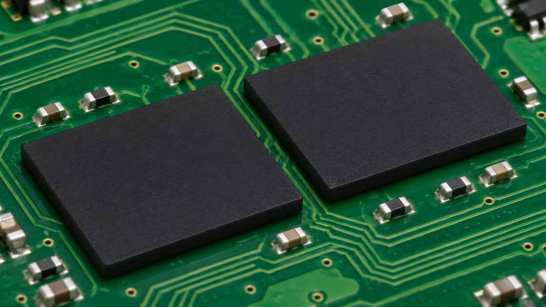
How Do You Verify PCB Trace Length Matching Before Manufacturing?

Verify PCB trace length matching by checking the configured rules, final routing reports, and physical geometry. Confirm whether the software evaluates length or delay and whether package and via contributions match the analysis assumptions.

PCB trace length matching, laboratory review of differential pairs and tuned routes

The release review should cover:

  • Constraint scope: Correct nets, pairs, groups, references, and endpoints.
  • Rule results: Matching limits, maximum length, and unresolved exceptions.
  • Physical routing: Transitions, reference continuity, and serpentine geometry.
  • Timing margin: Final path relationships against device requirements.
  • Channel behavior: Signal integrity analysis where the interface warrants it.
  • Revision consistency: Matching stackup and layout versions across analysis and fabrication files.

A CAD rule pass confirms compliance with the configured constraints. DFM checks manufacturing feasibility. Neither alone proves that the complete interface meets its timing requirements.

Preserve the approved material system, dielectric construction, and impedance targets during fabrication. Impedance testing verifies its specified characteristics; it does not independently certify length matching or interface timing.

FAQs About PCB Trace Length Matching

Q1: Can swapping data pins make length matching easier?

A1: Pin swapping can simplify routing when the device permits it, provided the schematic, pin mapping, and required configuration are updated consistently.

Q2: Can temperature changes affect trace-matching performance?

A2: Temperature-dependent material and device behavior can change timing margin, so designs with tight budgets should be evaluated across their specified operating range.

Q3: Does receiver training eliminate PCB length-matching requirements?

A3: Receiver training compensates within its supported range, while the board must still satisfy the device’s routing limits.

Q4: Can test points affect an otherwise matched signal path?

A4: Test-point pads and branches can introduce loading or stubs, so matching the main routes alone does not establish acceptable channel performance.

Q5: Can firmware correct excessive routing skew?

A5: Firmware can adjust timing only where the hardware provides suitable controls and sufficient adjustment range.

Q6: Should tuning patterns be placed beneath a connector or component body?

A6: They can be placed there when electrical spacing, reference continuity, and footprint restrictions permit, with nearby pads and holes included in the review.

For PCB fabrication or assembly support, send your Gerber or ODB++ files, approved stackup, impedance requirements, quantities, and BOM where applicable to sales@bestpcbs.com. Our engineering team can review manufacturing requirements and provide technical support and quotations for prototype and volume production.

You may also like

What Are the Main Transmission Line Termination Techniques?
Wednesday, September 2nd, 2026

The main transmission line termination techniques in PCB design are series, parallel, Thevenin, and AC termination. Series termination matches the source; the other three place a terminating network at the load. The choice depends on where reflections occur, how much current the driver can supply, and how quickly the receiver must reach a valid logic level.

A low clock frequency does not rule out the need for termination. A fast edge can reflect along a long trace before the voltage settles, while a short trace may work without a discrete resistor. Compare the signal’s fastest edge with the route delay, then check whether the receiver stays within its voltage and timing limits under the expected operating conditions.

Transmission line termination techniques, series at the source and parallel, Thevenin, or AC at the load.

What Is Transmission Line Termination in PCB Design?

Termination controls reflections by changing the impedance at a transmission line’s source or load. A PCB trace and its return path have a characteristic impedance, Z0. When a traveling edge reaches a different impedance, part of the voltage wave returns along the trace. Repeated reflections can cause ringing, overshoot, or a second crossing of a clock input’s threshold.

For an ideal resistive load, the reflection coefficient is:

ΓL = (ZL − Z0) / (ZL + Z0)

A matched load gives ΓL = 0. An open circuit gives +1, producing a reflected voltage of the same polarity; a short circuit gives −1, producing the opposite polarity. These are simplified limits. Receiver capacitance, package inductance, vias, and connectors make the real response frequency-dependent.

A load terminator absorbs the wave when it reaches the receiver. A source terminator absorbs the reflection when it returns to the driver. Both can control ringing, but the voltage seen along the trace differs between them.

When Does a PCB Trace Need Termination?

Analyze termination when the route delay is significant relative to the fastest rise or fall time. Clock frequency does not describe edge speed: a 10 MHz signal can still have subnanosecond transitions. Obtain the edge rate under the intended drive strength and loading, then estimate the complete source-to-load delay.

For example, a 100 mm route with an assumed propagation delay of 6 ps/mm has a one-way delay of 0.6 ns and a round-trip delay of 1.2 ns. With a 1 ns edge, the reflection takes long enough to affect the transition. With a 10 ns edge, the same route is electrically much shorter. The assumed 6 ps/mm is not a material specification; calculate the delay from the actual stackup.

Check three things before adding a resistor:

  • Interface requirements: inspect the transmitter and receiver documentation for internal termination, permitted networks, and drive settings. An external resistor may be unnecessary or harmful if matching is already on-chip.
  • Route topology: identify every receiver, connector, and branch. A source-terminated point-to-point result does not establish that a multi-drop bus will settle correctly.
  • Receiver margin: compare simulated threshold crossings and settling with the sampling window. For a clock, a second threshold crossing can matter even when the final voltage is correct.

How Do the Main Transmission Line Termination Techniques Compare?

The main trade-off among transmission line termination techniques is between source matching and load matching. Series termination adds little DC load at a high-impedance receiver. The load-end networks differ in their current demand, bias, and response to repeated transitions.

TechniqueMatching actionSelection condition
SeriesMatches the source to absorb the returning wave.One-way point-to-point route with a high-impedance receiver.
ParallelAbsorbs the arriving wave at the load.Load-end matching is needed and the driver supports the DC load.
TheveninProvides load matching at a chosen bias voltage.The interface needs both a terminating resistance and a defined bias.
ACProvides load matching during a limited transient interval.Continuous DC loading is undesirable and the signal pattern suits the RC network.

A one-way CMOS clock with one receiver is often a good starting point for series termination. If the interface specifies a load-end network, use that circuit as the starting point instead. Differential signaling describes the interconnect mode, not a fifth passive network; its termination follows the receiver and bus specification.

How Does Series Termination Work?

A series resistor combines with the driver’s output impedance to match Z0 at the source. Place it between the output pin and the main trace, with as little intervening copper as practical. The starting relationship is RS + Zdriver ≈ Z0.

In an ideal matched-source line with a high-impedance far end, the driver launches half of its open-circuit step voltage. At the far end, the positive reflection adds to the incident wave, so the receiver reaches the full step on the first arrival, after one one-way delay. The reflected wave then returns to the matched source and is absorbed. The receiver does not inherently have to wait for a round trip to reach the full level.

An input partway along a source-terminated trace sees the reduced step first and the returning reflection later. The intermediate voltage may sit near its switching threshold. This is why series termination works best with a single receiver at the far end, although receiver capacitance and package effects still need to be checked.

Series termination draws little steady-state current into a high-impedance load. Too much resistance can slow the edge and reduce timing margin. Check rising and falling transitions separately: the driver’s pull-up and pull-down impedances may differ. Analog Devices’ explanation of high-speed signal interfacing describes how the waves travel between the source and load.

How Does Parallel Termination Work?

Parallel termination places a resistor at the receiver or physical bus end so the incident wave sees a matched load. For a simple single-ended line, begin with RT ≈ Z0, connected to the reference required by the interface.

With a matched resistor, the arriving wave produces little reflection at the load. Keep the copper between the termination node and receiver short; any trace beyond the terminator is still unterminated. The connection to the reference also needs to be short, because its inductance weakens the match at fast edges.

The main cost is DC loading. A resistor to ground draws current in the high state; a resistor to the supply loads the low state. Calculate the actual loaded output voltage as well as resistor power. For an ideal 3.3 V source with 18 Ω output resistance driving 50 Ω to ground, the steady-state load voltage is only 3.3 × 50 / 68 ≈ 2.43 V, and the current is about 48.5 mA. Those assumed values illustrate why a correct impedance can still give an invalid logic level or excessive driver current.

Check the device’s output characteristics rather than relying on this simple resistive model. Even a smooth transition is unusable if the high level falls below VIH or the low level rises above VIL.

When Should You Use Thevenin Termination?

Use Thevenin termination when the interface needs load-end matching to a defined bias voltage. A resistor R1 connects the signal to VCC, and R2 connects it to ground. With low-impedance supply references, their parallel combination sets the terminating resistance:

Req = R1R2 / (R1 + R2)

VT = VCC × R2 / (R1 + R2)

For example, two 100 Ω resistors provide 50 Ω equivalent resistance and a 1.65 V unloaded bias from a 3.3 V supply. The undriven divider draws 16.5 mA. Driver current and resistor dissipation change when the signal is actively held high or low, so this is not the complete power budget.

Check the bias voltage as carefully as the resistance. A midpoint bias may leave the receiver at an invalid level while the line is idle or undriven. Resistor tolerance and reference noise affect both the bias and the match. Place both resistors at the load end, then check the high, low, and idle voltages against the receiver limits.

How Does AC Termination Work?

AC termination uses a series resistor-capacitor branch from the load to its reference. During a fast transition, the capacitor lets transient current flow through the resistor. After the capacitor charges, it blocks DC, reducing steady-state loading compared with a plain shunt resistor.

The match lasts only while the capacitor is charging. Too small a capacitor stops absorbing energy before the reflections settle. A larger one loads the line for longer, takes longer to recover, and draws more current during switching. The effective time constant depends on the impedances connected to the branch as well as its R and C values.

Test isolated edges, the fastest repeating pattern, and the longest allowed runs of identical bits. A network that damps an isolated edge may respond differently after several transitions. In each case, check the receiver thresholds and sampling window. TI’s comparison of differential termination techniques covers these AC-network limitations alongside resistive alternatives.

An AC termination branch connects from the load to its reference; it is not the same as a coupling capacitor inserted in the signal path. Do not substitute it for an interface-specified termination solely to reduce DC power.

How Is Termination Different for Differential Pairs?

A differential terminator matches the impedance seen between the two conductors. For a point-to-point LVDS link, a common implementation is one resistor across the receiver inputs. Its value follows the specified differential impedance and the receiver requirements.

Do not assume every differential pair needs 100 Ω. Some receivers already have a switchable internal resistor, while some buses need termination at both physical ends. Adding an external 100 Ω resistor across an enabled internal resistor of the same value gives a load of about 50 Ω, which can reduce the differential swing and overload the transmitter.

Place an external cross-pair resistor near the receiving pins with balanced connections. A resistor across the pair terminates the differential mode; it does not independently establish a common-mode bias or correct asymmetric routing. Split or biased terminations must follow the interface circuit rather than a generic substitution.

Analog Devices’ LVDS and M-LVDS implementation guide explains how point-to-point and multipoint layouts differ. Identify the physical line ends and allowed stubs before choosing the network; counting receivers alone is not enough.

How Do You Calculate Termination Resistor Values?

Start with the impedance match, then simulate nearby resistor values using the actual driver and trace. For series termination, subtract the driver’s effective output impedance:

RS ≈ Z0 − Zdriver

Worked example: assume a one-way point-to-point line, nominal Z0 = 50 Ω, estimated driver impedance = 18 Ω, and one high-impedance receiver. The starting resistor is 50 − 18 = 32 Ω. These are calculation assumptions, not measured board data.

Try 27 Ω, 30 Ω, 33 Ω, and 36 Ω in simulation. With the assumed driver, the total source resistances are 45 Ω, 48 Ω, 51 Ω, and 54 Ω. The 33 Ω resistor is closest to the nominal match; the simulations will show whether it also gives enough voltage and timing margin.

  • Model the driver: use the vendor’s validated IBIS model with the intended I/O settings. Check pull-up and pull-down behavior over process, voltage, and temperature; the assumed 18 Ω will not remain constant.
  • Vary the channel: include the specified impedance tolerance, receiver capacitance, resistor tolerance, packages, and vias. Compare the worst overshoot, undershoot, and settling time for each resistor.
  • Check the sampling point: reject values that cause extra threshold crossings or leave insufficient setup/hold margin. Choose a range that works across the tested conditions, rather than the value with the smoothest nominal waveform.

For a parallel resistor, start near Z0 and verify output current and loaded logic levels. For Thevenin termination, solve resistance and bias together. An AC branch also needs a capacitor chosen for the transient and pattern constraints. The device specification takes priority where it prescribes values or calibrated on-die termination.

Where Should Termination Resistors Be Placed?

Place source termination next to the driver and load termination next to the receiver or physical line end. Keep the unmatched copper segment short enough that its delay is small relative to the signal edge. The allowable distance depends on edge rate and stackup, so there is no universal millimeter limit.

  • Series network: route the output pin directly to the resistor, then continue with the main controlled-impedance trace. If the resistor cannot sit close to the pin, include that connecting segment in the simulation.
  • Parallel, Thevenin, or AC network: place the branch at the line end, with short connections to the receiver and reference. A long trace leading off to the resistor creates another segment that can reflect.
  • Differential or bidirectional link: preserve balanced pair connections and identify the physical ends. Follow the bus topology when either device can transmit.

Include pad expansions, neck-downs, return vias, and plane changes around the resistor in the channel model. The schematic treats the resistor as a lumped component, but its pads and connecting copper also affect the signal.

Transmission line termination techniques, resistor placement at the source and receiver with an unwanted long branch for comparison.

How Do Controlled Impedance and PCB Manufacturing Affect Termination?

A terminator must match the impedance of the manufactured trace, not just the nominal design value. Trace width, etched conductor shape, copper thickness, dielectric spacing, material Dk, and solder mask all affect impedance. Vias and reference-plane transitions add local discontinuities.

Consider a fixed 50 Ω load on a hypothetical line spanning 45–55 Ω. At 45 Ω, ΓL = 5 / 95 ≈ +5.3%; at 55 Ω, ΓL = −5 / 105 ≈ −4.8%. These are voltage-reflection coefficients for a single ideal resistive boundary, not measured overshoot or a board acceptance limit. They show why a nominal match still needs a tolerance analysis.

Before releasing the layout, agree on the controlled-impedance stackup and verification requirements: signal and reference layers, target impedance and tolerance, finished geometry, and a representative coupon. If the fabricator changes the dielectric or trace geometry, update the channel model and recheck the termination values.

A coupon TDR measurement checks that coupon’s impedance under the recorded test conditions. It cannot establish the timing of a complete route through connectors, vias, and loads. Use channel measurements to locate discontinuities, and check the powered receiver waveform separately. Keep the stackup revision, coupon identity, fixture details, and measurement conditions with the results so they can be compared with the simulation.

Fix a broken return path or long branch before tuning the resistor. Otherwise, a waveform that looks acceptable at one driver setting may fail when the load or temperature changes.

What Are the Most Common Termination Mistakes?

A resistor that matches the schematic may still perform poorly on the board. These symptoms help narrow down what to check:

  • A familiar resistor value still rings: confirm the current stackup and I/O drive setting. Reusing 22 Ω or 33 Ω from another board does not establish the same source impedance.
  • A low-frequency clock double-triggers: inspect its edge rate and receiver threshold crossings. Repetition rate alone does not rule out transmission-line behavior.
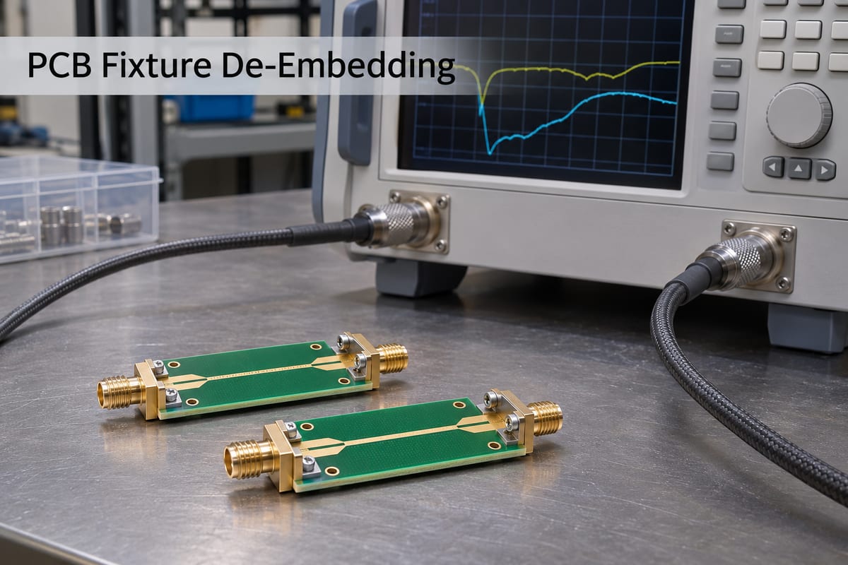
  • The edge becomes too slow: include driver impedance in the source match and check receiver capacitance. Adding a full Z0 resistor can introduce excessive source resistance.
  • Ringing remains despite a correct resistor: inspect the physical connection and probe setup. A long termination stub or probe ground lead can undermine the expected result.
  • Differential swing falls after assembly: check internal-termination settings and external population. Unintended parallel resistors may halve the intended load.
  • Typical simulation passes but hardware fails: compare model settings, actual geometry, supply conditions, and measurement loading. Retest operating corners before changing the resistor by trial and error.
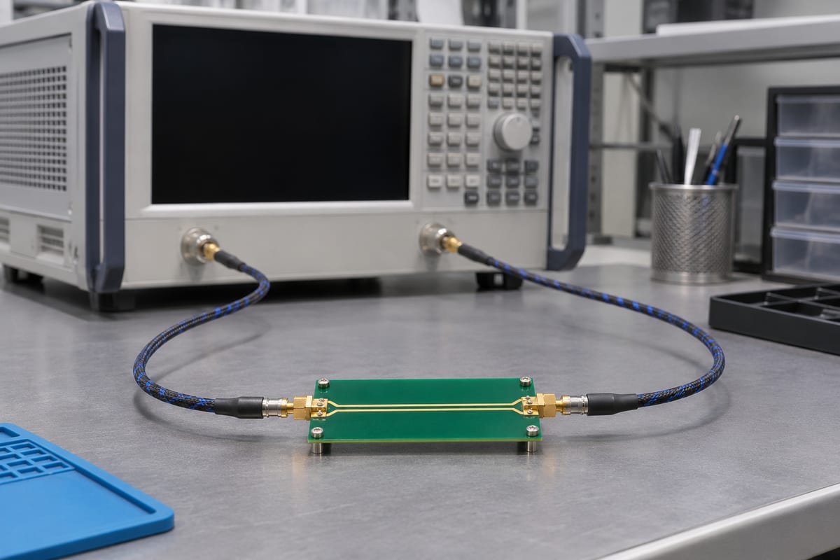
How Do You Choose the Right Transmission Line Termination Technique?

The right network keeps the receiver within its voltage and timing limits without overloading the driver. Work through the circuit in this order:

  1. Check whether termination is needed. Compare the fastest edge with the channel delay, then check the unterminated waveform against the receiver limits. This shows whether the route needs further termination analysis; clock frequency alone cannot answer that question.
  2. Check the topology and interface requirements. Mark the sources, receivers, physical line ends, and internal termination. Use the device documentation to identify which external networks are allowed and where they connect.
  3. Choose a network and calculate starting values. Decide whether the circuit needs source matching, load matching, a bias voltage, or temporary loading. Calculate the resistance and driver current, together with any bias or RC requirements.
  4. Simulate the routed board. Vary component values and operating conditions with the actual resistor placement, vias, and other discontinuities included. Keep the networks that meet the receiver’s voltage, threshold-crossing, and timing limits.
  5. Measure the prototype. Probe the receiver node with a suitable low-loading probe and compare the waveform with the simulation. Resolve any disagreement before finalizing the production BOM and I/O settings.

Keep the selected parts and I/O settings with the stackup revision, model versions, acceptance limits, and measured or simulated margins. After a layout or component change, these records show which assumptions need to be checked again.

FAQs About Transmission Line Termination

Q1: Should you terminate both ends of a transmission line?

A1: It depends on the interface and direction of transmission. Some bidirectional buses terminate at both physical ends; a one-way source-terminated point-to-point net typically uses a high-impedance far end. Adding a second network changes the loading and must be modeled.

Q2: Does DDR use the same termination on every signal?

A2: No. Data, strobes, clocks, and command/address signals can use different topologies and termination schemes. Follow the controller and memory generation’s routing rules and on-die termination settings; a generic 50 Ω or 100 Ω recommendation is insufficient.

Q3: What if driver impedance is already higher than Z0?

A3: A negative result from Z0 − Zdriver means a positive series resistor cannot create the desired source match. Recheck the model and permitted drive settings, then simulate another valid circuit rather than adding resistance automatically.

Q4: Must a termination resistor match 50 Ω exactly?

A4: First verify that 50 Ω is the correct target. The accepted resistor value depends on the termination type, device impedance, tolerance, and required margin. A nominally exact resistor cannot correct an incorrect stackup or a large local discontinuity.

Q5: How close is close enough to the pin?

A5: Use any device-specific layout limit first. Otherwise, model the segment between the pin and termination relative to the fastest edge. A fixed distance such as 5 mm is not universally safe across different edge rates and stackups.

Q6: Should you add optional termination footprints?

A6: They can make prototype tuning easier if placed at the correct boundary. Include the pads and unused branch geometry in the model, and document which parts are fitted so assembly does not create unintended double termination.

Conclusion

Start with the interface requirements and signal path, calculate the initial component values, then test the routed board. A nominal impedance match is only the starting point: the receiver must still see valid voltage levels and enough timing margin under the expected operating conditions.

Need a controlled-impedance PCB or assembly quote? Send EBest Circuit your Gerber or ODB++ files, proposed stackup, signal layers, impedance targets and tolerances, quantity, and required delivery date. Request a free DFM review and include any coupon and test-report requirements. For assembly, also send the BOM, placement data, and a clear list of which optional termination parts should be fitted.

You may also like