

PCB manufacturing PCB manufacturing
Home > Blog

Signal Integrity

Phase Noise Guide: Read, Measure and Compare Clocks
Saturday, November 21st, 2026

To compare phase noise, start with the carrier frequency, the offset range and the measurement conditions—not one impressive number. A clock with lower noise at one offset can still produce more integrated timing uncertainty in the band your receiver or converter actually uses.

This guide explains how to read a phase-noise plot, convert a defined noise spectrum into RMS jitter, and decide whether a measurement represents the oscillator or the instrument. The calculations are explicitly hypothetical; they are not measurements of a particular oscillator, PCB or customer’s product.
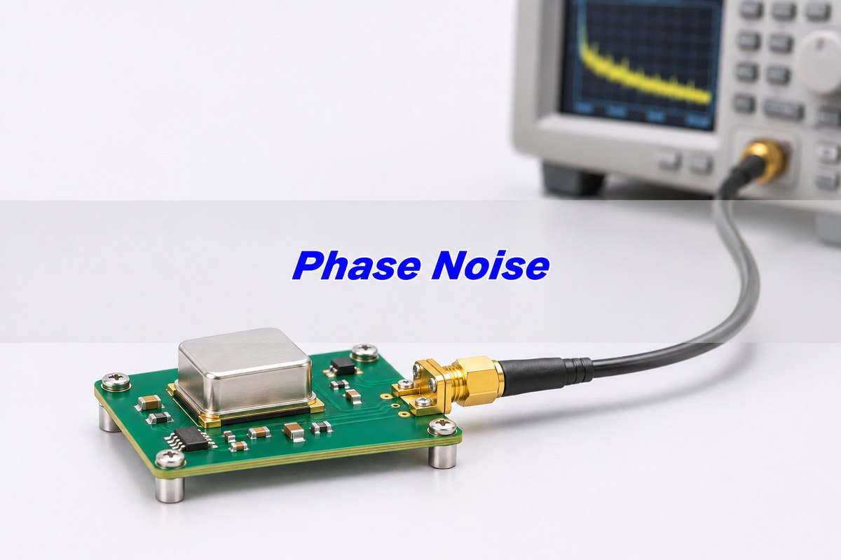
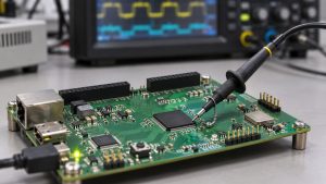
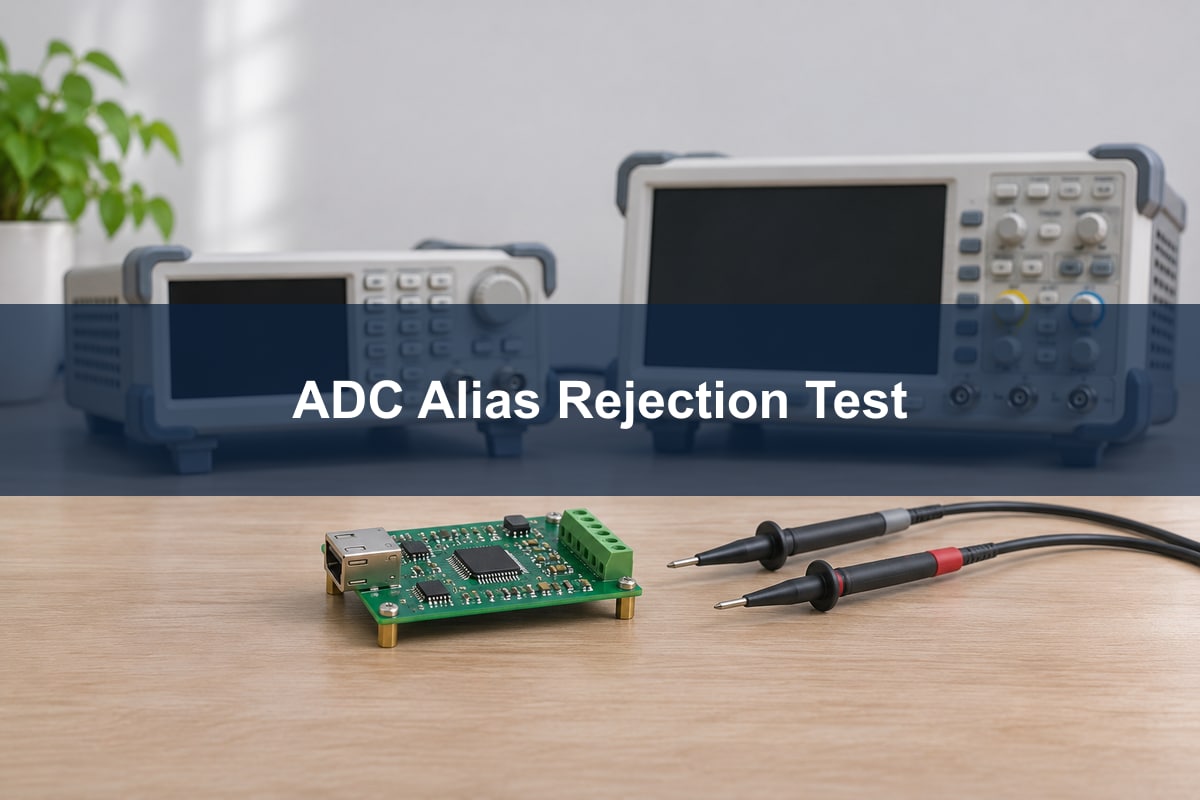
Phase Noise title above an illustrative oscillator PCB connected to generic test equipment
Illustrative clock-board measurement scene, not an instrument screenshot or verified DUT measurement.

What is phase noise?

Phase noise is short-term fluctuation in a signal’s phase. An ideal carrier would have perfectly predictable phase progression. A real oscillator departs from it, spreading noise around the carrier in the frequency domain and moving signal timing in the time domain.

A useful model is v(t) = A cos[2πf0t + φ(t)]. Here f0 is the carrier frequency and φ(t) is the phase fluctuation. This model separates phase variation from amplitude variation; a real measurement can contain both. Do not label every visible spectral skirt “pure phase noise” without checking the measurement method.

The practical question is where that noise hurts. A sampling clock changes when an ADC captures a signal. A receiver’s local oscillator can spread energy from nearby interference into the wanted channel. A PLL reshapes different noise contributions. Those are related effects, but their acceptance conditions are not interchangeable.

Phase noise units: what does dBc/Hz mean?

Single-sideband phase noise L(f) is noise power in a 1 Hz bandwidth at an offset f from the carrier, expressed relative to carrier power. Its usual unit is dBc/Hz. More-negative values mean lower noise density under the same conditions.

For example, “−140 dBc/Hz at 100 kHz offset, 100 MHz carrier” contains three essential facts. The carrier is at 100 MHz; the noise is examined 100 kHz away from it; the result is normalized to 1 Hz. It does not mean that the oscillator itself runs at 100 kHz or has −140 dBm of total noise.

Discrete spurs are different from a continuous noise density. Report a spur’s relative integrated power in dBc and its offset, and say whether the instrument includes it in integrated jitter. Copying a spur peak from a dBc/Hz display without knowing its bandwidth handling can create a misleading comparison.

Phase noise plot: read the offsets before the headline

The horizontal axis is usually logarithmic offset frequency, not the carrier frequency. The vertical axis is noise density. Read the conditions first, then examine close-in behavior, wider-offset noise and narrow spurs separately.

A better value at 10 kHz does not establish a better value at 1 MHz. If two curves cross, the application determines which region matters. Also check whether the plot represents a free-running oscillator, a locked PLL, an output buffer or an entire clock path. A datasheet’s best operating mode may not be your selected mode.
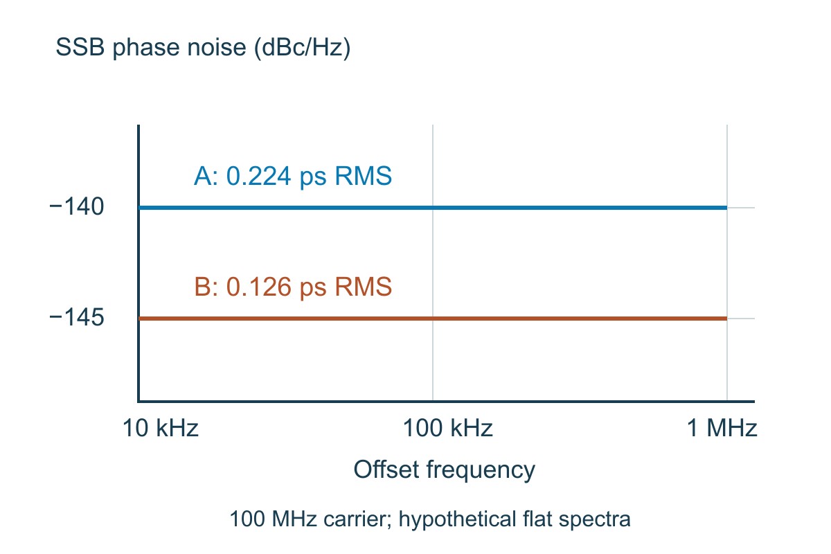
Hypothetical flat phase-noise spectra A minus 140 and B minus 145 dBc per Hz from 10 kHz to 1 MHz
Analytical comparison only: both examples use a 100 MHz carrier and the same 10 kHz–1 MHz integration band. Real oscillators need their actual spectra.

Before choosing a part, request the relevant plot or data table at your output frequency, supply, output format and loading. A single “typical jitter” value with no integration limits is insufficient to reproduce the result.

Phase noise vs jitter: which evidence do you need?

Phase noise retains information about where fluctuations occur in frequency. Integrated RMS jitter compresses a specified part of that spectrum into one timing number. Neither is automatically the better specification; they answer different questions.

Decision Phase-noise evidence Timing evidence
Compare RF local oscillators Noise at offsets related to channel separation and interference, plus spur limits A single integrated number can hide the important offset region
Budget sampling-clock uncertainty Integrate the relevant spectrum with the clock path’s filtering understood RMS clock jitter can enter a qualified converter noise calculation
Find edge-to-edge timing behavior Useful background, but not a substitute for all time-domain metrics Measure the specified TIE, period or cycle-to-cycle quantity
Compare supplier claims Match carrier, offsets, output mode and spur treatment Match integration limits and definition before comparing RMS values

Use the jitter measurement guide for the differences between TIE, period and cycle-to-cycle measurements. Converting phase noise to one RMS value does not make those quantities identical.

Phase noise to jitter: a calculation you can check

For small phase fluctuations with a consistently defined single-sideband spectrum, convert dB values to linear power before integrating:

σφ² = 2 ∫fLfH 10L(f)/10 df, then σt = σφ / (2πf0).

The factor 2 accounts for the two sidebands under this convention. Integrating dBc/Hz values directly, omitting the factor, or using the offset frequency in place of the carrier produces the wrong result.

Worked hypothetical example: let f0 = 100 MHz, L(f) = −140 dBc/Hz throughout 10 kHz–1 MHz, with no discrete spurs included. The bandwidth is 990,000 Hz. The linear density is 10−14/Hz, so phase variance is 2 × 10−14 × 990,000 = 1.98 × 10⁻⁸ rad². RMS phase is 0.000140712 rad; RMS time is 0.223951 ps, or approximately 224 fs.

Input or result Example A Example B
Carrier / offset band 100 MHz / 10 kHz–1 MHz 100 MHz / 10 kHz–1 MHz
Assumed flat SSB density −140 dBc/Hz −145 dBc/Hz
Calculated RMS time 0.224 ps 0.126 ps
What the result covers Only the specified hypothetical noise band The same band and assumptions, allowing a fair comparison

B’s 5 dB lower density reduces time RMS by a factor of 10−5/20 ≈ 0.562, not by “5 ps.” For a real sloping spectrum, integrate the actual linear data or a justified piecewise model. Do not stretch this flat example across an unmeasured band.

Choose fL and fH from the system requirement and transfer behavior. There is no universal “10 kHz–1 MHz” acceptance band. A tracking loop or clock input can weight noise differently; apply the appropriate transfer function when a rectangular integration window is not an adequate model.

Phase noise measurement with spectrum analyzer: check the floor

A direct spectrum-analyzer measurement compares nearby noise with the carrier and normalizes the result to bandwidth. Its usable range depends on dynamic range, analyzer local-oscillator noise and measurement settings. An attractive trace is not proof that those contributions are negligible.

Check input power, attenuation, reference level, offset range and the instrument’s noise-normalization method. Use the manufacturer’s phase-noise procedure rather than subtracting an arbitrary resolution-bandwidth number from a screen marker. Amplitude noise or overload can also invalidate a phase-only interpretation.

Here is a simplified illustration of floor contamination: independent noise powers of −140 and −150 dBc/Hz sum to −139.586 dBc/Hz, about 0.414 dB above the first contribution. Two equal −140 dBc/Hz contributions sum to −136.990 dBc/Hz, about 3.010 dB higher. This is a power-addition example, not a universal correction formula for every phase-noise instrument.

If the DUT result follows the analyzer floor, change to a validated lower-floor method or report the measurement limitation. Do not subtract almost equal traces and present the unstable difference as an accurate low-noise oscillator result.

Phase noise measurement cross correlation: what it removes

A two-channel phase-noise system observes the same DUT through two measurement paths. Cross-correlation can reduce uncorrelated noise added by the channels while retaining the DUT’s common contribution. More processing can improve sensitivity, at the cost of measurement time.
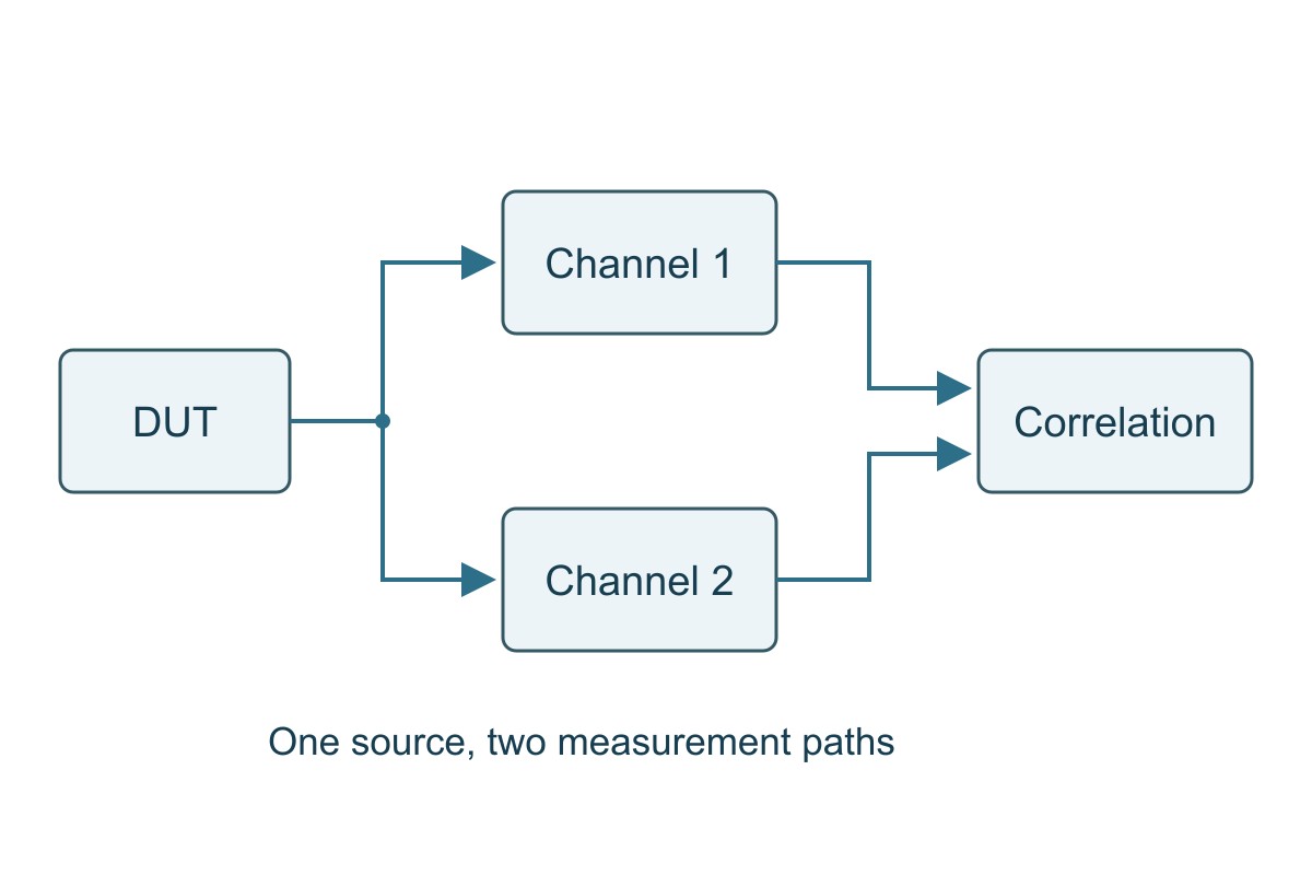
Simplified phase-noise cross-correlation setup with one DUT split into two measurement channels
Conceptual measurement paths. Actual instrument architecture and calibration follow the instrument documentation.

It does not remove real DUT noise. Nor does it automatically reject shared interference, common supply coupling or correlated errors. If a line remains while channel noise falls, investigate its origin rather than assuming enough averaging will erase it.

Record the correlation or averaging configuration with the result. Comparing a long, low-floor acquisition with a quick preliminary sweep without noting the difference can make an instrument setting look like a product improvement.

Where phase noise matters: applications and acceptance checks

ADC sampling clocks

The clock sets sampling instants; uncertainty becomes signal error. Use the noise delivered to the actual converter clock input, with the relevant filtering and bandwidth. For a sine-wave input, the jitter-only ceiling is SNR = −20 log10(2πfsignalσt).

Using example A’s band-limited clock contribution only, a 20 MHz input gives approximately 91.0 dB; a 100 MHz input gives approximately 77.0 dB. These are not complete ADC SNR predictions: aperture jitter, other clock noise outside the example band, distortion and converter noise remain. Verify the delivered clock and the converter spectrum under the intended input frequency, amplitude and configuration.

RF receiver local oscillators

The LO translates signals to another frequency. Noise around it can transfer interference energy into the wanted band, so the important offsets relate to the channel and blocker arrangement. Preserve wanted-channel sensitivity; control the noise contribution around relevant blocker separations, not merely the integrated number printed on a clock brochure.

For an illustrative blocker 1 MHz from the wanted signal, inspect the LO spectrum around the relevant 1 MHz offset and apply the receiver’s actual bandwidth and conversion behavior. A single spot value still does not establish total in-channel noise. Verify sensitivity or error performance with the specified wanted signal and blocker present, then repeat the comparison with identical receiver gain and bandwidth.

PLLs and clock-distribution boards

A PLL is not an all-purpose noise eraser. Reference-path noise and VCO noise have different transfer responses; changing loop bandwidth trades their contributions. An output buffer and the assembled clock path can add further noise.

Compare spectra before and after the PLL or buffer at the same carrier and load, and integrate with the system’s required weighting. Then verify lock behavior, output mode and relevant timing limits. If the operating mode uses deliberate spread-spectrum modulation, treat that separately; spread spectrum clocking is not equivalent to a lower random phase-noise floor.

Reducing phase noise: use a comparison worksheet

Begin with a repeatable baseline. Record output frequency, supply condition, load, temperature, measurement path, offsets, spur handling and integration settings. Change one suspected contributor at a time; otherwise a better trace does not tell you which change helped.

Observed evidence Controlled check Decision and next step
A narrow line appears near a switching-related offset Compare supply spectra and a verified alternate supply condition without changing other settings If both move together, investigate coupling; correlation alone is not final proof
PLL output is worse in part of the band Compare reference, VCO model and configured loop response Revisit loop trade-offs; do not simply narrow bandwidth on every design
Noise increases after a buffer or PCB path Match output format, loading and measurement reference plane before comparing Separate path-added noise from changed termination or analyzer settings
Result sits on the instrument floor Check a qualified lower-floor acquisition method Report a limit or repeat; do not release a claimed improvement without resolution

Example use: if a line appears at a suspected supply-related offset, record its offset and relative power, compare a controlled supply change, and repeat the original condition. If the line does not reproduce, do not close the investigation with “better decoupling fixed it.” Save the spectra and conditions that support the conclusion.

For acceptance, require the specified spot-noise mask, integrated jitter band and spur limits at the relevant clock output. A PCB fabrication pass alone cannot prove a populated oscillator circuit’s phase-noise performance. Agree the functional RF or clock test separately from bare-board acceptance.

Phase Noise FAQs

Is −140 dBc/Hz better than −130 dBc/Hz?

At the same carrier, offset and conditions, it is 10 dB lower noise density. It does not establish that the entire spectrum or integrated jitter is better.

Why does the integration bandwidth change jitter?

The integral counts noise within the selected band. Changing its limits changes the included power. Use the application’s required band or transfer weighting, and state it with the result.

Can I integrate phase noise in dB directly?

No. Convert L(f) to linear power density, integrate over frequency, apply the SSB convention and convert RMS phase to time using carrier frequency.

What RMS jitter does the example −140 dBc/Hz spectrum produce?

Approximately 0.224 ps for a flat spectrum from 10 kHz to 1 MHz at a 100 MHz carrier, excluding spurs. Different limits or spectrum shape give a different answer.

Does the ADC calculation use the clock frequency as the input frequency?

No. The jitter-only SNR formula uses the analog input signal frequency. The phase-to-time conversion separately uses the clock carrier frequency.

Should spurs be included in phase-noise-derived jitter?

State the requirement and the instrument’s treatment. Report discrete spurs separately in dBc and identify whether the integrated result includes them; do not silently compare different conventions.

Does cross-correlation remove the oscillator’s noise?

No. It helps reduce uncorrelated measurement-channel contributions. Noise common to the paths, including the DUT contribution, remains.

Can a better PCB layout guarantee lower phase noise?

No. Layout can affect coupling, supply integrity and clock-path behavior, but the oscillator, PLL, buffers and test setup also matter. Demonstrate improvement with matched measurements rather than a layout-only claim.

Technical References

Custom RF PCB Manufacturing with Prototype and Assembly Support

Need a custom RF PCB or assembled clock board? EBest Circuit supports RF PCB fabrication, prototype builds and PCB assembly. File review connects your material and stackup requirements with the actual manufacturing and assembly scope, helping avoid a bare-board quotation that leaves the populated-board requirements unresolved.

Send your Gerber or ODB++ files, stackup, material requirements, impedance targets and quantity to sales@bestpcbs.com for a quotation. For PCBA, add the BOM, placement data and required functional test. Tell us which RF or clock measurements the project needs so the test scope can be evaluated explicitly—without assuming that a fabrication check guarantees phase-noise performance.


You may also like

Spread Spectrum Clocking Guide: EMI vs Timing Margin
Saturday, November 21st, 2026

Spread spectrum clocking, or SSC, deliberately varies a clock’s frequency so its spectral energy is distributed over a range instead of concentrated at fixed frequencies. It can lower measured emission peaks, but it also changes the timing seen by the receiving circuit. Use it only after confirming that the entire clock path supports the modulation, then verify both emissions and system operation.

The first decision is not “how much spread gives the biggest dB improvement?” It is “what frequency range, modulation rate and timing behavior can this system accept?” This guide explains those parameters, compares center and down spreading, and gives a calculation and release worksheet. Numerical examples are analytical teaching cases, not measurements of a manufactured PCB.

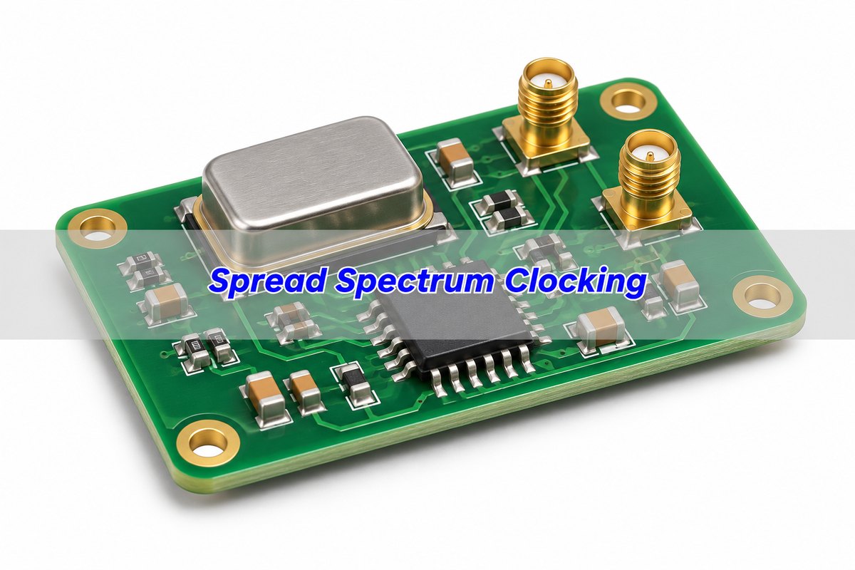
Spread Spectrum Clocking title over an illustrative clock generator PCB
Illustrative clock hardware. The image does not establish an implemented modulation profile or a measured emissions reduction.

Spread spectrum clocking meaning: intentional frequency variation

A fixed clock produces spectral components around its repetition frequency and harmonics. SSC modulates that repetition frequency in a controlled way. A receiver measuring a limited frequency band may then observe less energy concentrated in one peak. The technique redistributes energy; it does not make every source of electromagnetic interference disappear.

Distinguish intentional modulation from unwanted random jitter. Both affect edge timing, but they have different descriptions and validation requirements. An interface designed to track a documented SSC profile can behave differently from a precision sampling circuit that needs a low-noise, spectrally clean clock.

It is also different from fixing the radiation path. A poor return path, an unsuitable connector transition or a cable carrying common-mode current can still radiate. Correct those design issues rather than using SSC to hide an unexplained failure at one analyzer setting.

The practical benefit is additional emission margin when the signal and system support it. The trade-off is a wider frequency excursion and a timing condition that must remain inside the receiver’s allowed behavior.

Spread spectrum clock modulation: read the four key parameters

Define nominal frequency, actual minimum and maximum frequency, modulation rate and modulation profile. A percentage is not enough because vendors can define “depth” as one-sided excursion, total span or a field interpreted differently by the selected mode.

Parameter Practical meaning and analytical example
Nominal clock frequency 100 MHz in this example; the unmodulated period is 10 ns. This is not the modulation rate.
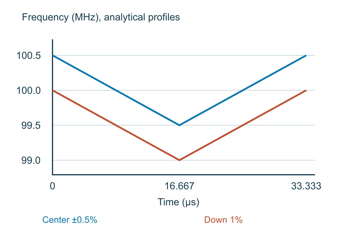
Center spread ±0.5% 99.5–100.5 MHz, a total frequency span of 1 MHz.
Down spread 1% 99–100 MHz, also a 1 MHz span, but without exceeding the nominal upper frequency in the idealized profile.
Down spread 0.5% 99.5–100 MHz, only a 0.5 MHz span. It is not the same excursion as center spread ±0.5%.
Modulation frequency Assume 30 kHz: one modulation cycle takes 33.3333 µs. Many 10 ns clock cycles occur during that sweep.
Modulation profile A triangle, sinusoid or another supported profile determines how frequency moves with time. Use the device’s defined profile rather than assuming all SSC generators behave alike.

Frequency and period move inversely. For the center-spread example, the period at 100.5 MHz is 9.95025 ns, while at 99.5 MHz it is 10.05025 ns. For the 99–100 MHz down-spread example, the periods range from 10 ns to 10.10101 ns. These are instantaneous-period endpoints, not RMS jitter values.

Write the frequency endpoints explicitly in a design review. That makes a factor-of-two depth misunderstanding visible before anyone programs a register.

Center spread vs down spread: compare the actual frequency limits

Center spreading moves above and below a nominal frequency. Down spreading remains at or below the nominal frequency in its specified modulation profile. The choice depends on frequency ceilings, receiver tracking and application requirements, not on which name sounds quieter.

Mode for a nominal 100 MHz clock Decision, cost and boundary
No intentional spreading Use when the receiver or precision task does not support SSC. Timing still contains real oscillator and distribution imperfections; “SSC off” does not mean zero jitter.
Center ±0.5%, 99.5–100.5 MHz Provides a 1 MHz excursion around nominal. The receiving path must tolerate the upper frequency as well as the lower one; check absolute limits and all additional tolerances.
Down 1%, 99–100 MHz Uses the same idealized 1 MHz span without the center mode’s upward excursion. Its lower average frequency and longer period endpoints may affect throughput or synchronization.
Down 0.5%, 99.5–100 MHz Has half the span of the center ±0.5% example. Do not claim equal spectral spreading merely because both settings contain “0.5%.”

TI’s SPRABY0A configuration report cautions that center spread raises the highest interface frequency, while down spreading lowers average frequency. Those observations explain the basic trade-off; the report’s specific SoC settings are not universal operating limits for other devices.

Analytical triangular frequency profiles comparing center spread 99.5 to 100.5 megahertz and down spread 99 to 100 megahertz over 33.333 microseconds
Two idealized profiles with the same 1 MHz total span and a 30 kHz modulation rate. The frequency limits differ; this is not a measured clock trace.

Spread spectrum clocking configuration: start at the receiver

Map the clock tree from source to every receiving function. Identify where modulation is generated and what each intervening buffer, divider, multiplier or PLL does with it. A control labeled “spread spectrum” does not establish which branches are affected.

  1. Read the receiver/interface requirements: allowed clock frequency range, SSC mode and depth, modulation rate, jitter definition and clock architecture.
  2. Identify the actual clock path and the devices that must accept the modulated input. Check configuration and operating modes, not just component names.
  3. Translate the proposed percentage into minimum and maximum frequency and period. Include the applicable source accuracy and other tolerances using the required method.
  4. Check the generator’s exact parameter units and profile. Confirm whether a software “depth” field means half-span or full span in that mode.
  5. Program only a supported configuration, read it back where possible and measure the output. Verify startup, lock and the required operating transitions.

A downstream PLL may track some modulation or filter it according to its design and operating conditions. Do not assume that modulation applied at a base clock reaches every multiplied clock unchanged. Conversely, do not assume that every PLL removes it. The exact architecture and documented behavior determine what must be measured.

If a board exposes an SSC option in firmware or BIOS, identify the clock domain and manufacturer’s intended setting before changing it. An overclocking anecdote is not a qualified configuration for a production interface.

Spread spectrum clock generator: verify the setting, not just the feature name

SSC may be integrated into a processor clock block or generated by a dedicated device. Choose by output format, voltage, frequency range, supported modulation, startup/configuration behavior and the receiving system’s requirements. A longer list of SSC modes is not proof of a better fit.

For a concrete documentation example, TI’s CDCE(L)913 datasheet, revision SCAS849I of August 2024, lists center and down settings separately in Table 7-2. A setting shown as ±0.5% in center mode is shown as −0.5% in down mode. The corresponding total frequency spans differ, as the calculation above demonstrates.

That family also illustrates why part suffixes matter: CDCE913 and CDCEL913 have different output-supply options. Verify the exact part, output levels, pins, loading and configuration rather than treating a similar model name as a drop-in replacement. The example identifies a documentation issue, not a recommendation for every clock tree.

Keep the selected configuration file or register record with the hardware revision. If production programs nonvolatile settings, define how programming success is verified. A correctly assembled board with the wrong saved clock configuration can still be the wrong product.

Spread spectrum clocking PCIe: the clock architecture matters

Do not enable SSC on a PCIe reference simply because another PCIe board uses it. Common-clock and separate-reference arrangements have different requirements, and both link partners and the clock distribution must support the intended arrangement.

TI’s November 2023 application note SNAA386 describes a common-clock SSC example with 0% to −0.5% down spread and a 30–33 kHz modulation frequency. At an ideal nominal 100 MHz, that percentage corresponds to 99.5–100 MHz before other tolerances are considered. The same note distinguishes separate-reference architectures.

Use those figures as a scoped manufacturer explanation, not a replacement for the applicable PCI-SIG specification and device documentation. Verify the required generation, topology, reference architecture and allowed SSC settings for the actual link. In particular, do not infer independent-clock compatibility from a successful shared-clock example.

Validate the link using the prescribed timing and compliance method, relevant traffic and operating conditions. Successful enumeration is a useful first check, not complete proof of long-term margin or compliance.

EMI measurement with SSC: keep the receiver settings comparable

The observed benefit depends on the emitted spectrum and how the measurement receiver observes it. Record resolution bandwidth, detector, sweep/dwell behavior, operating mode, cables, enclosure and measurement geometry. Changing these between SSC-off and SSC-on tests can create a misleading comparison.

A simple energy-per-band estimate helps explain the mechanism. Suppose an idealized total power is distributed uniformly across 1 MHz and the observation bandwidth is 120 kHz. The ratio is 1,000/120 = 8.3333; 10 log10(8.3333) = 9.20819 dB. This is a teaching estimate under a uniform-power assumption, not a predicted compliance improvement.

Actual modulation has a profile and spectral structure; peaks are not necessarily uniform across that span. Receiver detector and timing behavior, source harmonics and the coupling path also matter. Analog Devices’ spread-spectrum discussion uses a similar simplified bandwidth argument and distinguishes estimates from measured peak behavior.

Measure the complete required emission range and operating modes with the applicable method. A reduced peak at the fundamental does not prove every harmonic or nearby band improved. Record the worst relevant results and margin; do not promise a fixed dB reduction from a percentage setting alone.

Spread spectrum clocking applications: verify the benefit and the cost

Display and digital clock domains. SSC can be a supported way to reduce clock-related peaks. For example, TI publishes an AM62x display-subsystem procedure tied to that SDK and clock configuration. Confirm the panel/interface and receiver allow the resulting frequency excursion, then check the required display timing, image stability and operating transitions as well as emissions. Do not copy a platform-specific setting into an unrelated SoC.

Serial interconnects. Use the allowed reference-clock architecture and modulation profile. Verify both link partners, timing measurements and relevant traffic/error behavior. Preserve the clock settings in the test record. For measurement definitions, use the site’s jitter measurement guide; an intentional low-frequency modulation should not be compared with an unlabeled RMS jitter number.

Switching-power synchronization. Some regulators support frequency spreading or an appropriate modulated synchronization input. Check the regulator’s allowed synchronization range and tracking behavior, then test regulation, ripple, transients and the required emissions. A modulation profile suitable for a digital reference is not automatically suitable for a power converter.

Precision sampling and spectral measurements. Be cautious when the sampling clock’s spectrum directly affects the measured signal. ADI AN-1386 explains how clock spectral imperfections influence ADC output spectra. Establish whether deliberate spreading is compatible with the converter and measurement task, then verify the relevant SNR, spurs, resolution and timing behavior. There is no blanket rule that every ADC must use SSC or that none can; the system requirements decide.

In each application, the release decision has two sides: did the required emission result improve, and does the product still meet its functional and timing requirements? Passing only one side is not a completed design change.

Example clock path from reference through an SSC generator to a downstream PLL and clock domain with verification points A and B
Conceptual clock path: at A, verify the generated profile; at B, verify downstream behavior. The diagram does not imply that every PLL passes or removes SSC.

Spread spectrum clocking checklist: release a measured configuration

Use this worksheet before enabling SSC in a design release. The first row is a worked numerical check; the other rows require actual device and test evidence.

Input or evidence Decision and next action
Example: nominal 100 MHz, center ±0.5%, 30 kHz triangle Calculate 99.5–100.5 MHz, 1 MHz span and 33.3333 µs modulation period. Confirm the receiving path allows these conditions before programming.
Receiver and interface documents Record applicable versions, architecture and allowed profile/range. If SSC support is not established, do not assume it.
Clock-tree and configuration revision Identify which outputs are modulated and how downstream devices behave. Read back settings and measure the relevant output nodes.
EMI comparison record Keep detector, bandwidth, setup and product mode comparable. Record actual worst relevant results, not just one improved trace peak.
Functional and timing results Check the application-specific link, display, regulator or sampling requirements under the required conditions. Resolve degradation before release.

If increasing spread reduces a spectral peak but breaks a receiving clock constraint, use a smaller supported setting or another EMI-control method. Do not trade an unexplained functional failure for a better-looking emissions screenshot.

Spread Spectrum Clocking FAQs

Does SSC reduce the total energy generated by a clock?

Its basic purpose is redistribution over frequency, not a universal reduction of total emitted energy. The measured peak benefit depends on the source, coupling path and receiver settings.

Are center ±0.5% and down 0.5% the same spread?

No. At 100 MHz, the center example spans 99.5–100.5 MHz, while the down example spans 99.5–100 MHz. Compare actual endpoints and the manufacturer’s parameter definition.

Does 30 kHz modulation mean the clock runs at 30 kHz?

No. It means the frequency-sweep pattern repeats every 33.3333 µs. A nominal 100 MHz clock still has clock periods near 10 ns.

Does down spread guarantee that the real clock never exceeds nominal?

The ideal modulation profile has that upper endpoint, but the actual clock also has specified accuracy and other tolerances. Evaluate the complete allowed frequency range, not just the nominal profile.

Can I enable SSC in BIOS without checking the clock domain?

Do not assume the option affects only the intended branch. Use the system manufacturer’s documentation and validate the affected interfaces and operating modes.

Will a downstream PLL remove all SSC?

Not necessarily. Its tracking and filtering behavior depend on the design and settings. Check the documented path and measure the relevant output.

Does the 9.20819 dB calculation guarantee that EMI improves by that amount?

No. It assumes uniform distribution over 1 MHz and a 120 kHz observation band. Actual profile, spectral peaks, detector behavior and coupling require measurement.

Is an operating PCIe link enough to release an SSC change?

No. Confirm the specified clock architecture, timing/compliance requirements and required operating/error tests. Initial link operation is only one check.

Custom High-Speed PCBs with Engineering DFM Support

Need custom PCBs for a timing-sensitive product? EBest Circuit supports multilayer and high-frequency PCB manufacturing with engineering DFM review. Reviewing the stackup and controlled-impedance geometry before fabrication helps align the manufactured construction with your released design; PCB assembly support keeps board and component requirements connected.

Send your Gerber or ODB++ files, stackup, material and impedance requirements, quantity and delivery needs to sales@bestpcbs.com. Add the BOM and placement data for assembly. Request a manufacturing review and project-specific quotation with construction and inspection requirements clearly identified. Clock configuration and product EMC qualification remain part of the system validation plan.

Technical References

You may also like

Jitter Measurement Guide: RMS, Peak-to-Peak and TIE
Saturday, November 21st, 2026

For a useful jitter measurement, define the timing event, reference, measurement bandwidth and reported statistic before comparing numbers. A result of “10 ps jitter” is incomplete: 10 ps of period RMS, time-interval-error RMS and observed peak-to-peak timing variation can describe different behavior.

This guide covers electronic clock and data-edge timing, not packet-delay variation in a network. It explains the main measurements, compares instruments and shows how to use the results for clock distribution, serial links and ADC sampling. All numerical examples below are synthetic calculations, not measurements from a customer PCB.

Jitter Measurement title over an illustrative clock PCB and bench oscilloscope arrangement
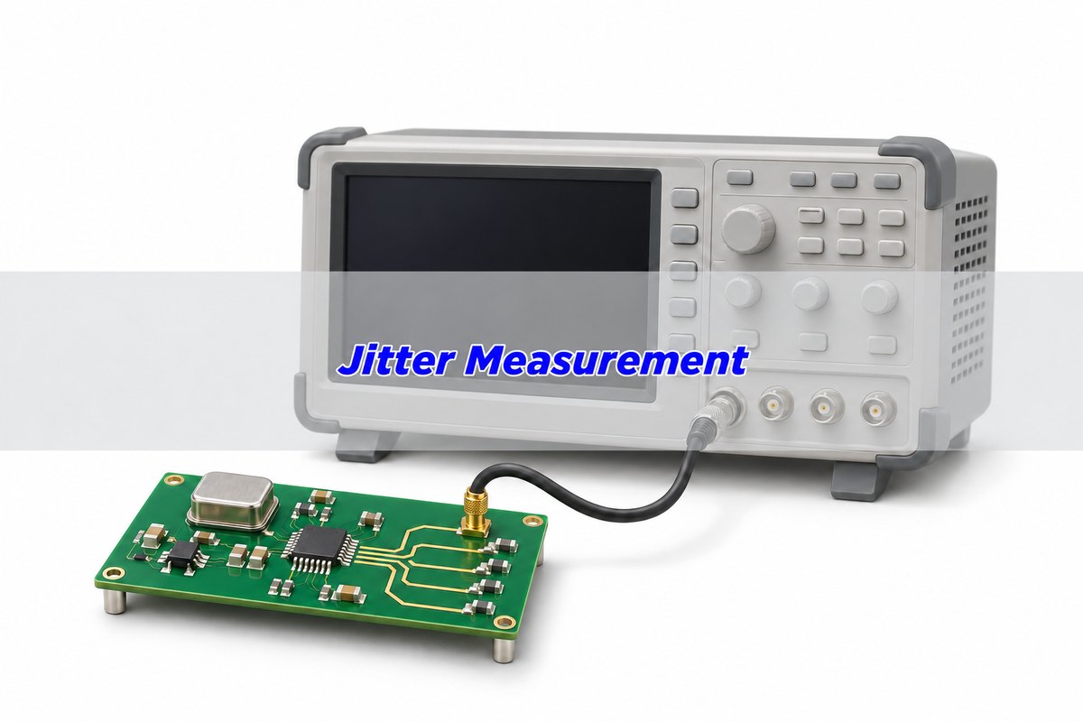
Illustrative measurement setting. Instrument appearance and the pictured PCB do not establish a measured jitter value.

Jitter measurement unit: seconds and unit intervals

Timing jitter describes variation in when an edge reaches a defined event, usually a voltage-threshold crossing, relative to the chosen timing reference. State the threshold, edge polarity and reference because changing them can change the result. A fixed propagation delay and a variation of that delay are not the same quantity.

Time results commonly use seconds, picoseconds or femtoseconds: 1 ps = 10⁻¹² s and 1 fs = 10⁻¹⁵ s. A unit interval, UI, expresses time relative to the symbol interval used by the link. For an assumed 1 Gb/s NRZ stream, UI = 1/(10⁹ s⁻¹) = 1 ns = 1,000 ps. A 20 ps timing width is therefore 0.02 UI, or 2% of that UI.

Do not use the clock frequency to define data UI without checking the interface. A DDR or multilevel link can have a different relationship between clock, symbol rate and bit rate. Use the applicable interface definition before converting a compliance limit.

Also separate skew from jitter. A consistent arrival-time difference between two clock branches is a relative timing offset; variation over time is another effect. A design may need both checks, but combining them into one unlabeled “jitter” number obscures what should be corrected.

Period jitter vs TIE: the same edges produce different numbers

Let tn be the measured time of the nth rising edge and T the chosen reference period. Period error is (tn+1 − tn) − T. Time interval error, TIE, compares an edge with its reference position: tn − (t0 + nT) for the fixed reference used in this example.

Cycle-to-cycle period variation compares consecutive periods. It highlights a different behavior from the accumulated displacement shown by TIE. A reference recovered from the signal can track some timing variation; its recovery method and bandwidth therefore belong in the measurement definition.

One synthetic edge record Derived quantity and interpretation
Reference period: 1,000 ps Ideal edge times: 0, 1,000, 2,000, 3,000 and 4,000 ps.
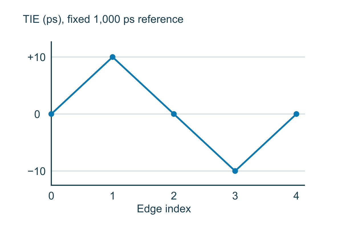
Actual times: 0, 1,010, 2,000, 2,990 and 4,000 ps TIE: 0, +10, 0, −10 and 0 ps relative to that fixed reference.
Measured periods 1,010, 990, 990 and 1,010 ps; mean period is 1,000 ps.
Period errors +10, −10, −10 and +10 ps; their RMS is 10 ps.
Adjacent-period differences −20, 0 and +20 ps. These are cycle-to-cycle differences, not the TIE sequence.
TIE population statistics for these five edges Mean 0 ps, RMS about the mean 6.32456 ps, observed peak-to-peak 20 ps. Five edges do not characterize a production clock’s distribution.

The example explains why two instruments can disagree without either being numerically broken: they may be reporting different observables or using different references. First align the definitions; only then investigate acquisition or instrument errors.

Synthetic TIE values at five edge indices: zero plus ten zero minus ten and zero picoseconds
The same five-edge teaching record used in the table. This is a calculated TIE sequence, not an oscilloscope capture.

RMS jitter vs peak to peak jitter: compare matching statistics

RMS about the mean describes the spread of timing-error samples. For N samples ei, calculate the square root of the mean of (ei − mean(e))² when that is the specified population statistic. Some tools use a sample-standard-deviation estimator or report RMS without removing the mean; record the actual definition.

Observed peak-to-peak is the largest recorded value minus the smallest. In the five-edge example, +10 − (−10) = 20 ps. Its ratio to the 6.32456 ps RMS is a property of this tiny record, not a universal conversion factor.

Under a Gaussian random-jitter model, the theoretical tails are unbounded. Collecting more edges can expose larger extremes even when the underlying RMS remains similar. Therefore a measured peak-to-peak value needs a record length or event count. A total-jitter estimate at a specified BER needs the statistical model and BER as well.

Do not multiply every RMS jitter result by six, fourteen or another remembered factor. Such factors have specific assumptions and probability definitions; mixed random and deterministic jitter does not become a Gaussian distribution merely because a histogram looks smooth.

Jitter measurement oscilloscope: control the acquisition first

At the bench, identify the actual measurement node and required loading. A probe or cable can alter the waveform, and the oscilloscope’s own vertical noise and timebase behavior can contribute to the reported crossing times. Choose a setup capable of resolving the required effect, not only one whose screen shows a clean clock.

  1. Confirm clock rate or data pattern, signal amplitude, termination and threshold. Record rising, falling or both edge selections.
  2. Define the timing reference. For recovered-clock measurements, retain the recovery method and loop settings required by the application.
  3. Set and record acquisition rate, analog bandwidth, filtering and record length. Verify that the waveform and edges are adequately captured for the chosen method.
  4. Inspect the timing trend and distribution as well as summary values. A time-dependent modulation can disappear inside one aggregate number.
  5. Repeat under controlled conditions to check repeatability, then change one suspected influence at a time.

Begin by ruling out a measurement artifact. If moving the probe ground connection changes the result substantially, investigate the connection and loading before redesigning the oscillator. If changing the threshold produces a large timing shift, inspect waveform shape, noise and edge slope rather than assuming the timebase is the sole cause.

For a hypothetical uncorrelated-error model, suppose measured timing RMS is 12 ps and a separately characterized measurement contribution is 8 ps under matching conditions. Quadrature subtraction gives √(12² − 8²) = 8.94427 ps, not 12 − 8 = 4 ps. This estimate is valid only when the components and statistics support that model; correlated errors or unmatched bandwidth invalidate the simple subtraction. Near the instrument floor, report the limitation.

Jitter measurement techniques: match the instrument to the question

A time-domain waveform, an oscillator phase-noise spectrum and a bit-error test expose different aspects of timing behavior. Choose the method by the decision you need to make, then state its limitations. An instrument’s ability to display a result does not establish that its noise floor is low enough for your clock.

Technique Use it for this decision; verify these conditions
Real-time oscilloscope timing analysis Examine individual edges, TIE trends, distributions and relationships with data or supply events. Verify probing, timing reference, event count and instrument contribution.
Phase-noise analysis Characterize oscillator noise versus offset frequency and derive integrated phase/time jitter over a stated band. Verify carrier frequency, integration limits, spur treatment and analyzer floor.
Bit-error-rate testing Evaluate link errors or timing margin with a defined pattern, receiver setup and test duration. It does not identify every physical cause and is not interchangeable with a clock RMS specification.
Simulation Compare modeled channel, driver, receiver and noise effects before hardware changes. Validate inputs and compare with measurements; a simulated eye is not a production measurement.

For phase-derived time jitter, the small-phase relation is σt = σφ/(2πf0), with phase RMS in radians and carrier frequency f0 in hertz. A hypothetical integrated phase RMS of 0.001 rad at a 100 MHz carrier gives 1.59155 ps RMS. The integration band must accompany that result; a single phase-noise value at one offset cannot supply the whole integrated jitter.

Analog Devices’ MT-008 explains the phase-noise integration workflow. Use an appropriate implementation and its documented treatment of sidebands and spurs rather than integrating displayed dB numbers directly. Do not compare two integrated results from different offset bands as though they represented the same measurement.

Random jitter vs deterministic jitter: keep the model visible

Random jitter, RJ, is commonly treated with a Gaussian model and summarized by an RMS quantity. Deterministic jitter, DJ, represents bounded systematic contributions such as periodic modulation, duty-cycle distortion or data-dependent effects. The decomposition is an analysis model, not a photograph of physically isolated noise sources.

A periodic component in a timing trend suggests a repeatable influence worth correlating with known activity. A data-dependent timing shift suggests examining pattern history and channel response. Neither observation uniquely names the failed component. Change the suspected influence in a controlled test and check whether the corresponding timing feature changes.

Keysight’s dual-Dirac description explicitly distinguishes RJ RMS from a model-dependent DJ(δδ) quantity used to estimate TJ at a specified BER. Do not relabel that DJ estimate as the directly observed peak-to-peak span of all deterministic behavior. Keep the instrument algorithm, settings and target BER with the report.

For a serial link, a favorable decomposition result does not override the receiver’s required compliance method. Follow the applicable interface procedure, including pattern, recovery and equalization settings. There is no single general-purpose IPC jitter limit for every PCB interface.

Noise and slew rate: why the crossing time changes

Near a locally linear threshold crossing, a small voltage error can produce a timing error approximately equal to δt ≈ δV / |dV/dt|. The relation explains an important distinction: limiting bandwidth can reshape or delay a repeatable edge, while noise acting on that edge can change when its threshold is crossed.

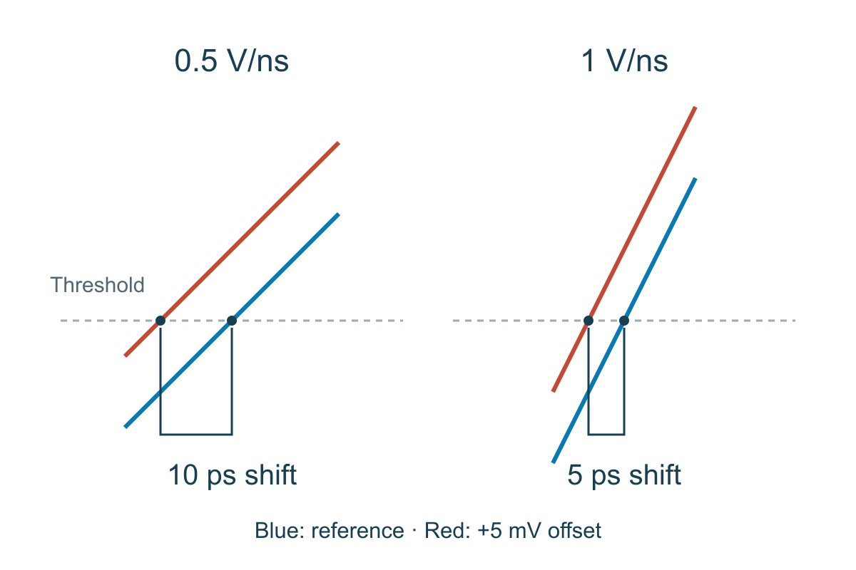
Assume 5 mV RMS voltage noise at the crossing and a local slope of 0.5 V/ns. The approximate noise-derived timing RMS is 0.005/0.5 ns = 10 ps. If the same noise acts on a 1 V/ns slope, the estimate is 5 ps. These are local illustrative calculations, not a complete instrument uncertainty budget.

A bandwidth limit is therefore not automatically “jitter = 1/bandwidth.” But changing bandwidth can change both edge slope and admitted noise, so its net effect must be evaluated under the actual setup. Reducing noise by filtering while making the edge much slower is a trade-off, not a guaranteed improvement.

Analytical comparison of five millivolt noise producing ten picosecond timing shift at half a volt per nanosecond and five picoseconds at one volt per nanosecond
Local linear-crossing example with the same 5 mV noise input. It illustrates a mechanism, not measured total jitter.

When comparing board revisions, preserve amplitude, threshold, load, measurement bandwidth and probe arrangement. Otherwise an apparent improvement may come from the measurement setup rather than the circuit. Recheck the waveform and the timing distribution after any change.

Clock jitter applications: what to measure and how to judge it

Clock distribution. A clock feeding several devices must satisfy the relevant input timing and signal-level requirements at the receiving pins. Measure the selected period or TIE quantity under the stated load and operating condition. Examine branch skew separately. Compare the results with the receiving device’s actual specification, not a universal “good clock” number.

Serial PCB links. Preserve enough horizontal and vertical margin for the specified receiver and link conditions. Evaluate the required patterns, channel condition, clock recovery and equalization; inspect error behavior or the specified eye/jitter metrics. Keep termination and fixture boundaries controlled. The site’s signal integrity software guide explains how to choose a modeling workflow, while the eye diagram guide covers the display’s interpretation. An eye that looks open in a short acquisition is not proof of an arbitrarily low BER.

ADC sampling. Sampling-time uncertainty changes the sampled voltage most strongly where the input waveform is steep. For a sinusoidal input and the usual small, uncorrelated timing-error approximation, the jitter-only limit is SNRjitter = −20 log10(2π fin σt). Here fin is the analog input frequency, not the sampling-clock frequency.

With an assumed total sampling jitter of 1 ps RMS, a 20 MHz sine input gives a calculated jitter-only limit of 78.0158 dB; a 100 MHz input gives 64.0364 dB. The higher-frequency input is more sensitive to the same time uncertainty. These values are not predicted total ADC SNR: quantization, thermal noise, distortion and other effects remain.

To verify the ADC application, use the intended input frequency and amplitude, clock path and acquisition method, and compare the appropriate spectral performance with the device/system requirement. Combine independent jitter contributions by root-sum-square only when the assumptions hold. A low-jitter oscillator datasheet does not include every effect added by the board and converter.

Jitter measurement checklist: make the report reusable

Use this worksheet before accepting a comparison or releasing a design change. The first row is filled with the synthetic record above so the calculation can be reproduced. Fill the remaining rows with the actual project conditions and criteria; blank fields are unresolved information, not passes.

Record this input or condition Decision and next action
Example: fixed 1,000 ps period; TIE [0, 10, 0, −10, 0] ps Mean 0 ps; population RMS about mean 6.32456 ps; observed peak-to-peak 20 ps. This verifies arithmetic, not a device’s long-term distribution.
Node, load, threshold and edge polarity Match the intended receiver or measurement definition. Resolve differences before comparing board revisions.
Metric, reference and recovery settings Distinguish period, cycle-to-cycle and TIE. Retain the method and any loop/filter settings.
Bandwidth, record length and event count Compare like acquisitions. Do not call a larger observed peak-to-peak value a degradation until the measurement conditions match.
Instrument contribution and repeatability Show the measurement can resolve the required margin. Report floor/uncertainty limitations rather than subtracting incompatible values.
Requirement, test procedure and result Identify the device/interface document and its version. Use its applicable acceptance method; record any extrapolated BER model separately from direct observations.

A useful conclusion says which timing requirement was tested, under which conditions, how much margin remains and what was not established. If the report only says “jitter improved,” it is not yet a dependable engineering handoff.

Jitter Measurement FAQs

Can I compare 10 ps RMS with 10 ps peak-to-peak?

No. They are different statistics. Obtain the same metric, reference, bandwidth and event count or model definition before comparing the two results.

Why does peak-to-peak jitter increase with a longer record?

A longer observation can include more extreme events. Under a Gaussian RJ model the tails are theoretically unbounded, so an observed peak-to-peak value is tied to the acquisition, not a guaranteed worst-case bound.

Is period jitter the same as time interval error?

No. Period error concerns each edge-to-edge interval; TIE concerns edge displacement from the selected reference. The five-edge example gives 10 ps period-error RMS but 6.32456 ps TIE RMS.

Does lower oscilloscope bandwidth always reduce timing jitter?

No. It can reduce admitted noise while also slowing the crossing slope. Compare the resulting timing error under the required bandwidth and signal conditions rather than assuming one direction of change.

Can a phase-noise analyzer replace every oscilloscope jitter test?

No. Phase-noise analysis is useful for oscillator spectral behavior and integrated jitter, while a waveform capture can expose edge-by-edge and data-correlated behavior. Select the method required by the application.

What information is needed with an integrated RMS jitter value?

Include carrier frequency, offset-frequency integration limits, spur treatment and the instrument/method. A single phase-noise point does not define the integral.

Why can the same 1 ps jitter matter more to a higher-frequency ADC input?

The sinusoid’s slope increases with input frequency. In the stated jitter-only model, 1 ps gives 78.0158 dB at 20 MHz but 64.0364 dB at 100 MHz; total ADC performance includes other limits.

Does a better jitter result prove the PCB construction is acceptable?

No. It supports the defined timing test. The fabricated board still needs the agreed construction, dimensional, connectivity and other applicable acceptance evidence.

Custom High-Speed PCBs with Engineering DFM Support

Ready to manufacture the board behind your timing-sensitive design? EBest Circuit supports custom multilayer and high-frequency PCB manufacturing with engineering DFM review. Reviewing the stackup and controlled-impedance geometry before fabrication helps keep the released construction aligned with your design assumptions; PCB assembly support can connect the fabrication and BOM discussion in one project.

Send your Gerber or ODB++ files, stackup, material requirements, impedance notes, quantity and delivery needs to sales@bestpcbs.com. Add the BOM and placement data for assembly. Request a manufacturing review and quotation with the construction, inspection requirements and open engineering questions clearly identified.

Technical References

You may also like

Vector Fitting S-Parameters: From Data to Validated Models
Saturday, November 21st, 2026

Vector fitting turns sampled frequency responses into a rational model built from poles and residues. For PCB interconnects, that model can help a circuit simulator use measured or electromagnetic-extracted S-parameters in transient analysis. The important qualification is this: a smooth-looking fit is not automatically an accurate, passive or correctly connected simulation model.

Start with the complete complex data and a defined simulation task. Fit only after checking ports, reference impedance and frequency coverage; then validate the exported model, not just the fitting plot. This guide explains that workflow and provides an analytical one-pole example for checking units and numerical results. The example is synthetic, not a PCB measurement or a benchmark of any fitting package.

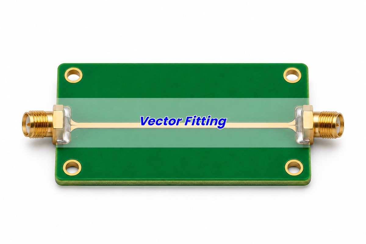
Vector Fitting title over an illustrative PCB interconnect coupon with two coaxial connectors
Illustrative interconnect coupon. A fitted model represents the response at defined ports; the picture is not measurement evidence.

What is vector fitting?

Vector fitting approximates complex frequency data with a mathematical function that can be evaluated between samples and represented in a circuit-simulation workflow. It is useful when a measured or extracted interconnect is known by its terminal response rather than by a simple schematic.

A PCB trace, connector transition or package interconnect may be represented by an S-parameter matrix over frequency. A transient simulator still needs a numerical representation it can combine with drivers, receivers and terminations. A rational macromodel is one route; using the simulator’s direct S-parameter or convolution capability is another. Choose the route the target simulator supports and validate the result in that environment.

Representation Choose it for this job; check this limit
Sampled S-parameter file Exchange terminal frequency-response data. The receiving simulator must define interpolation, extrapolation and time-domain handling; the file alone is not a complete driver/receiver model.
Vector-fitted rational model Create a compact pole-residue representation for a supported simulation workflow. Check model order, residual error, physical constraints and export compatibility.
Known-topology equivalent circuit Use when physically meaningful RLC or transmission-line elements capture the required behavior. Do not force an oversimplified topology to explain a complex multiport structure.

For a short, simple interconnect, an adequate transmission-line model may be easier to inspect. For a complicated multiport response, a fitted model can be more practical. Neither option recovers missing measurement information or proves the structure behaves linearly at every drive level. Keep the characterization conditions with the model.

Vector fitting algorithm: what the iterations change

The algorithm relocates poles iteratively, then determines the residues and other selected terms for the resulting pole set. SINTEF’s algorithm description explains that the repeated subproblems are linear; this is more structured than drawing a smooth curve through magnitude points.

Think of poles as common dynamic features and residues as the contribution of each feature to an individual response. For a multiport network, sharing poles across responses provides one coordinated model rather than unrelated scalar curves. The residues can differ for S11, S21 and the other matrix entries.

Three choices still belong to the engineer: what data to include, how much model complexity to allow and which errors matter to the application. A numerical stopping condition says the algorithm stopped according to its rules. It does not say the input data are correct or that an omitted resonance has become irrelevant.

If a fit changes drastically when the initial settings change, investigate order, frequency sampling, noise and the data boundary. Preserve the original file and settings so you can compare runs. Do not repeatedly increase complexity until one plot looks convincing without knowing which result improved.

S parameter rational fit: prepare the complete complex input

Use the full complex responses required by the network model, with consistent port definitions and reference conditions. Fitting only S21 magnitude discards phase, reflections and coupling information that can matter when the model is connected to a real circuit.

Before fitting, identify each port’s physical location, signal/reference relationship, ordering and reference impedance. Confirm whether the data represent the bare trace, fixture-plus-trace or a de-embedded structure. A fitted model cannot correct a port swap that was never detected.

Record the frequency unit and range, number of samples, DC treatment and any preprocessing. Check both magnitude and phase for discontinuities or unexpected behavior. For detailed file interpretation, use the site’s Touchstone file guide; the fitting package should receive the same intended network, not a differently normalized or reordered version.

For a hypothetical four-port differential interconnect, prepare all 16 complex S-matrix entries at the defined frequency samples. Do not assume that fitting one through path establishes the other reflection and coupling paths. Whether symmetry or reciprocity can reduce independent information depends on the actual characterized structure and the model formulation.

Extrapolation needs separate attention. If the data begin above DC, the fitter does not magically know the DC behavior. If the target edge excites frequencies beyond the measured band, an in-band match does not establish the missing response. Obtain justified additional data or limit the model’s use; do not label extrapolated behavior as measured.

Poles and residues: read the model parameters

A common rational form is H(s) = d + s e + Σ rk/(s − pk), where s = σ + jω and ω = 2πf. The poles pk and residues rk describe frequency-dependent terms; d is constant and e is a proportional coefficient. The selected representation and simulator determine which terms are supported and appropriate.

The crucial unit distinction is between f in hertz and angular frequency ω in radians per second. Substituting f directly for ω moves the numerical corner by a factor of 2π. For a real-valued time response, complex terms must be handled with the required conjugate structure. Check the package’s representation instead of manually deleting a conjugate term because its plot seems redundant.

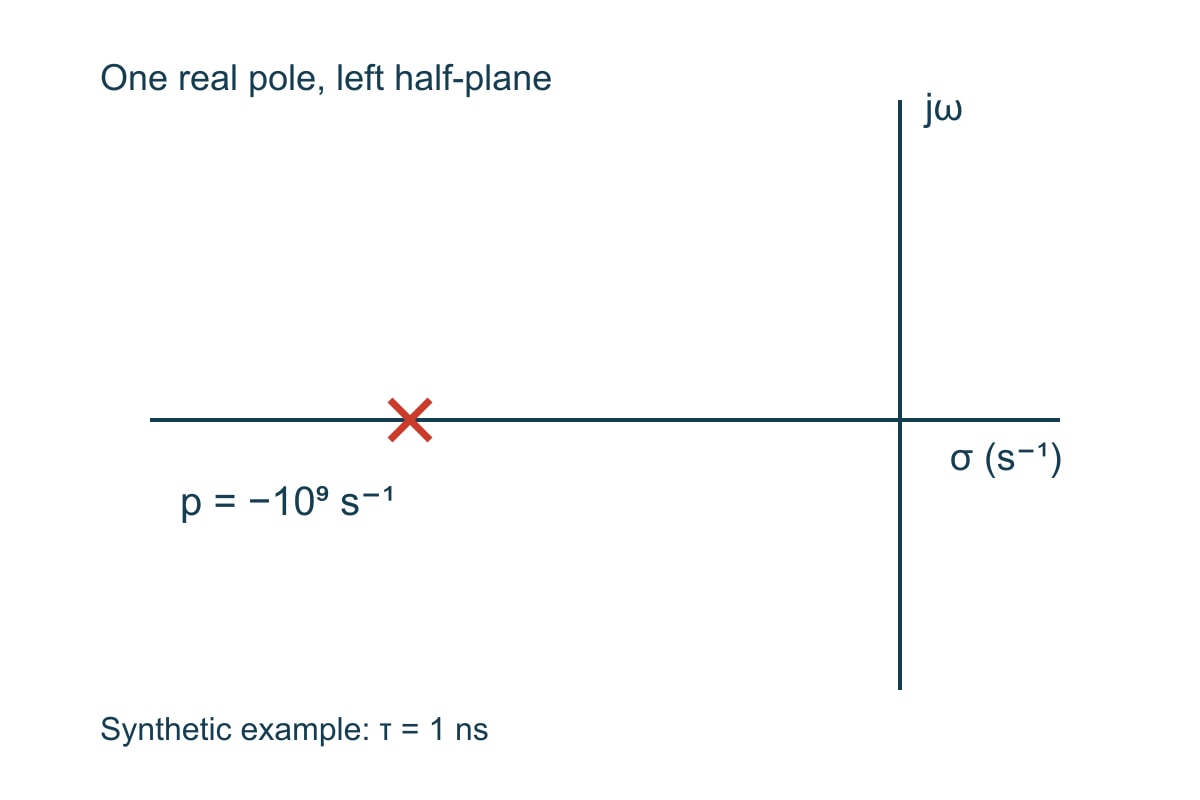
Here is a deliberately simple synthetic function: H(s) = 1/(1 + sτ) with τ = 1 ns. It is equivalent to H(s) = 10⁹/(s + 10⁹). The pole is p = −10⁹ s⁻¹, the residue is r = 10⁹ s⁻¹ and d = e = 0. This is a test function for learning and validation, not an extracted PCB channel.

Complex s plane showing a single real pole at minus one billion per second in the left half plane
Synthetic one-pole example. The pole is negative on the real axis; the frequency-response evaluation follows s = jω, not s = jf.
Quantity in this example Value and meaning
Time constant τ 1 ns; explicitly chosen teaching input.
Pole and residue p = −10⁹ s⁻¹ and r = 10⁹ s⁻¹; their ratio gives unit DC response for this function.
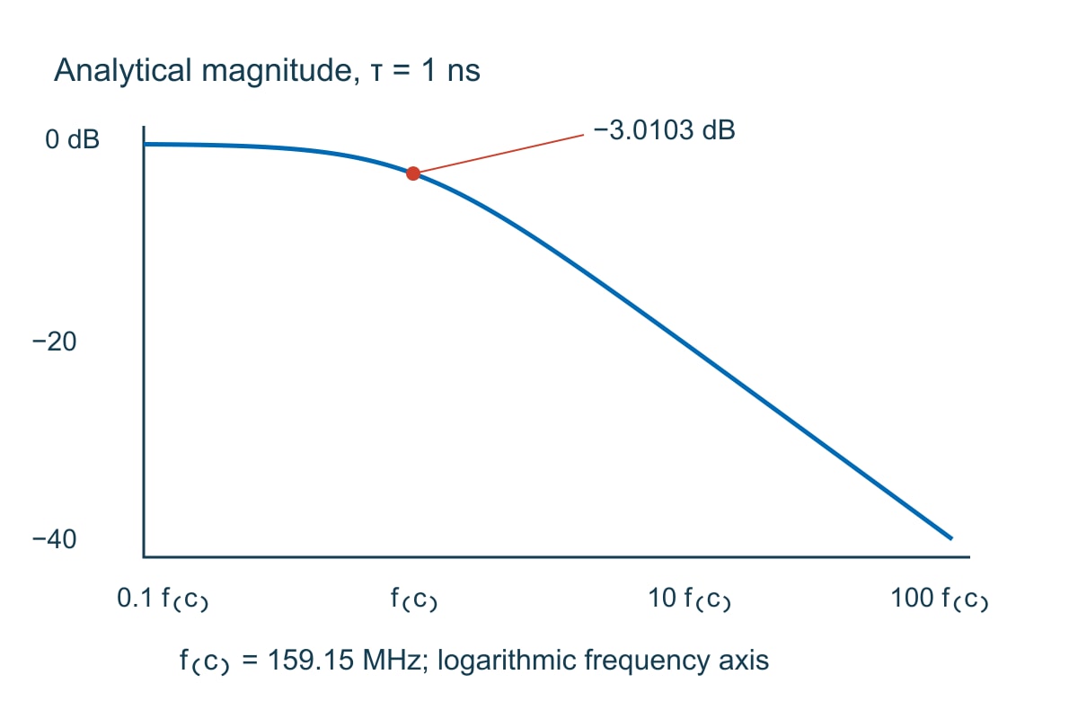
Corner frequency fc 1/(2πτ) = 159.154943 MHz, rounded to 159.15 MHz in the plotted label.
Magnitude and phase at fc 1/√2 = 0.70710678, or −3.01030 dB, with −45° phase.
Magnitude at 10 fc 1/√101 = 0.0995037, or −20.0432 dB.
Unit-step response at t = τ 1 − exp(−1) = 0.63212056. This checks the same analytical function in the time domain.

This example also shows why a pole’s numerical value is not its corner frequency in hertz: 10⁹ s⁻¹ corresponds here to 159.15 MHz, not 1 GHz. Compare any exported implementation against these analytical values before trusting the more complicated network workflow.

Model order: add complexity only when it improves the required result

Model order controls how much dynamic behavior the rational representation can describe. Too little order can miss structure; more order increases computation and can fit noise or poorly justified detail. There is no universal pole count for “a PCB model.”

Start from the response shape and the target application. Compare at least two reasonable settings using the same input data, weighting and evaluation frequencies. Inspect local residuals around resonances, reflections and low-amplitude coupling paths, not only a global average.

Use the one-pole function above as a controlled test: its analytical rational structure contains one real pole. Adding several poles should not be necessary to represent that exact noiseless function, although a numerical implementation may still return small numerical differences. If a simple test needs many modes to hide a unit error, increasing order is solving the wrong problem.

A long interconnect with substantial delay is different. Delay contributes phase that can demand a more complicated finite-order approximation over a wide band. Review the fitter’s documented delay handling or consider the simulator’s supported direct-data route. Do not claim that a higher pole count automatically makes the time-domain result more physical.

Passivity enforcement: recheck accuracy after changing the fit

Stable poles and passivity are different requirements. Stable poles concern the model’s internal dynamics; a passive network must not generate energy through its ports. SINTEF’s constraints discussion explicitly calls for a passivity check in S-, Y- and Z-parameter modeling rather than treating stable pole placement as sufficient.

For the intended passive interconnect, evaluate the complete fitted network with the applicable normalization and method. A satisfactory S21 magnitude alone cannot establish multiport passivity. The site’s S-parameter passivity guide covers that check in more detail.

The scikit-rf 2.1.0 passivity example demonstrates that a fit can look close to passive sampled data and still violate passivity. Its enforcement step also warns that the DC point cannot always be preserved. The engineering consequence is simple: enforcement is a model change. Compare its new complex responses, DC behavior and application result with the original requirements.

If enforcement needs large corrections, return to the input data, order and model assumptions. Do not repeatedly repair a model until the warning disappears while ignoring the response it now represents. An enforced model can satisfy a physical constraint and still be too inaccurate for the intended decision.

Vector fitting Python vs MATLAB: choose a usable delivery route

Choose an implementation by whether it can read your data, represent the required terms, test the relevant constraints and deliver a model accepted by the target simulator. A Python or MATLAB label does not establish accuracy or compatibility by itself.

scikit-rf provides documented vector-fitting functionality and examples in Python. SINTEF provides MATLAB-oriented implementations and documentation. Confirm the exact package version, dependencies, licensing and supported export path you intend to use; do not assume that every feature mentioned on a project website is present in every downloaded version.

A practical trial has three stages. First evaluate the analytical one-pole function to verify units and response interpretation. Next use a small representative network with known port mapping and compare the complex fitted data. Finally import the exported model into the actual simulator and check the same terminations and output quantities that matter to the project.

For a team handoff, deliver the input checksum or controlled revision, settings, software version, fitted model, validation record and port map together. A netlist without its reference impedance and port mapping may be syntactically valid but still be the wrong network. Compare the available signal integrity software workflows before choosing the model delivery route; verify the actual export in your receiving simulator.

RMS error and model validation: check the decision, not just the average

Use RMS error as one summary of residuals, then inspect where the error occurs and whether it changes the engineering result. A small matrix-wide value can hide an important local error in a weak coupling response or a narrow resonance. Define the error metric and weighting before setting an acceptance limit.

For a scalar response, one useful complex RMS definition is the square root of the mean of |Hfit − Hreference|² over the stated samples. That is not the same as RMS error in decibels or an RMS phase error. Record which definition the tool reports. Do not borrow a numerical “good fit” threshold from a demonstration and treat it as a release standard.

Analytical magnitude response for a one nanosecond first order function with 159.15 megahertz corner and minus 3.0103 decibel point
Analytical reference, not a measured or fitted result: H(s) = 1/(1 + s × 1 ns). Plot, table and calculations use the same input.

In a PCB channel application, preserve the through-path loss, phase and relevant reflections under the actual terminations; validate timing or eye results separately with appropriate endpoint models. In a coupled multiport application, check the weak paths and port coupling that determine the interference budget. In a passive filter model, resolve the transition and resonant features that set the filter decision. One average error cannot replace all three application checks.

Use this release worksheet after fitting and again after export. The first row demonstrates the numerical check. The remaining rows require project-specific inputs and criteria; they are not automatic pass/fail claims.

Input or check Expected decision and next action
Synthetic τ = 1 ns; evaluate at 159.154943 MHz Reference magnitude 0.70710678 and phase −45°. A factor-of-2π frequency discrepancy means check hertz/angular-frequency conversion before fitting real data.
Port map, reference impedance and characterization boundary Match the intended network. Resolve swaps, normalization changes or fixture inclusion before model approval.
Complex residuals across the required band Compare local and summary errors with the application’s allocated tolerance. Missing out-of-band evidence limits the permitted use.
Pole structure and applicable physical constraints Use documented checks for stability, realness and passivity where appropriate. Re-evaluate accuracy after any enforcement.
Exported model in the target simulator Reproduce reference frequency responses and the required time-domain checks with the stated terminations. Import success alone is not validation.

Vector Fitting S-Parameters FAQs

Can I fit an active device with vector fitting?

A rational approximation can represent active-device small-signal frequency responses, but do not enforce passive-interconnect behavior on an intentionally active model. Preserve the characterization conditions and understand what the linear model cannot represent, including nonlinear compression or a changing operating point.

Do I need to measure DC for every fit?

Not every task requires a measured DC point, but the low-frequency behavior must be justified for the intended simulation. Distinguish an added estimate from a measurement and check its effect on the time-domain result.

Why should phase be retained if I only care about insertion loss?

A transient network model needs the complex response. Different phase behavior can produce different delays and waveforms even when magnitude is similar. Fitting magnitude alone does not define the same causal dynamic model.

Does a lower RMS error always justify a higher-order model?

No. Determine whether the improvement occurs in the required responses and survives validation, rather than fitting noise or irrelevant samples. Compare runtime, constraints and the actual design result, not just one decreasing number.

Can vector fitting fix a wrong calibration plane?

No. It can approximate the response supplied to it, including fixture effects or calibration errors. Correct or explicitly include the characterization boundary before interpreting the model as a bare PCB structure.

Does passivity enforcement preserve all original data?

No. Enforcement changes the approximation and may alter DC or local response values. Recheck the changes against the error allocation and the intended simulation after enforcement and export.

How many responses are in a four-port S matrix?

There are 4 × 4 = 16 complex entries at each frequency. Physical symmetry or reciprocity can relate entries in an applicable structure, but the port map and model still need to preserve the required network behavior.

Does a fitted channel prove the fabricated PCB meets its specification?

No. A model represents particular input data and assumptions. Fabrication acceptance requires the agreed drawing, stackup, test conditions and evidence from the relevant produced boards or coupons. Simulation does not replace that evidence.

Custom High-Speed PCBs with Engineering DFM Support

Ready to turn a validated interconnect design into hardware? EBest Circuit provides custom PCB manufacturing and engineering DFM support. Reviewing the released stackup, controlled-impedance structures and fabrication files together helps expose build assumptions before they become a mismatch between your model and the manufactured board.

Send your Gerber or ODB++ files, stackup, impedance requirements, quantity and target delivery to sales@bestpcbs.com. Include the required coupon and test-report details. Request a fabrication review and quotation with construction, acceptance evidence and any open technical items clearly identified.

Technical References

You may also like

Signal Integrity Software: Choose Tools That Fit Your PCB
Friday, November 20th, 2026

Choose signal integrity software by the decision you need to make, not by the most impressive 3D plot. A tool for exploring a driver and a transmission line, a tool for extracting a PCB interconnect, and a tool for checking an equalized serial channel solve different parts of the problem. The useful choice is the one that accepts your real models and geometry, predicts the receiver behaviour you care about, and leaves a result you can verify.

If you are moving from PCB layout into signal integrity, start by listing the interface, available device models, channel construction and required pass criteria. This guide explains how those inputs change the tool you need. The numerical examples are teaching calculations, not measured boards or benchmark results from the software products discussed.

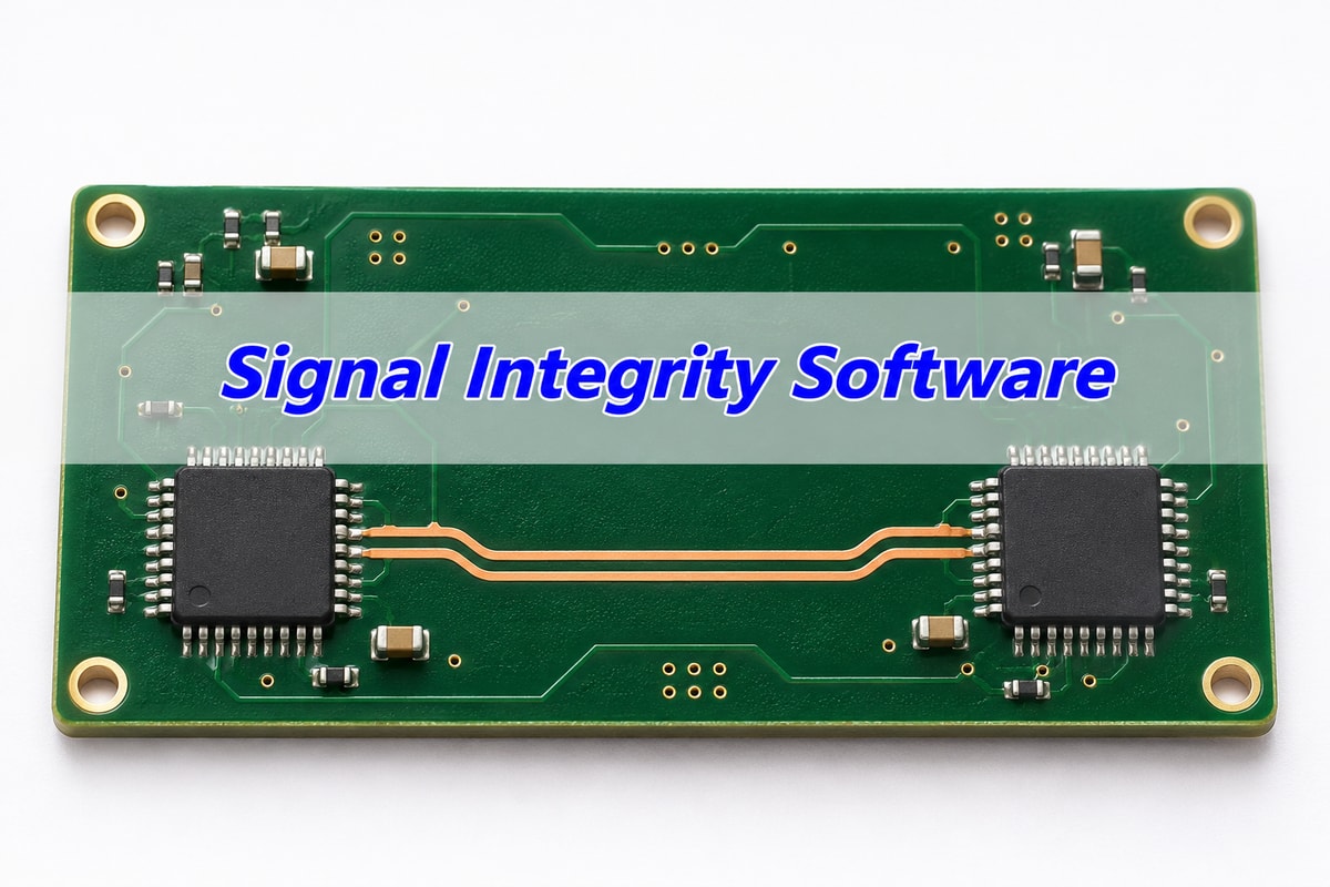
Realistic PCB digital interconnect illustration with two generic integrated circuits and the title Signal Integrity Software
Illustrative product rendering. A physical PCB channel needs both an interconnect model and appropriate transmitter and receiver models.

What is signal integrity analysis?

Signal integrity analysis asks whether an electrical signal arrives at the receiver with enough voltage and timing margin to be interpreted correctly. It examines effects such as reflections, loss, crosstalk and timing variation. It does not normally simulate the complete logic or firmware running inside a complex IC.

Think of a digital output driving a trace into a receiver. The driver has a finite output impedance and edge shape. The route, vias, connector and package alter the waveform. The receiver then applies its input behaviour and timing requirements. A perfect square-wave source driving an ideal wire leaves out most of what you wanted to check.

Also separate clock rate from edge rate. A low-frequency control signal can still launch a fast transition. Whether transmission-line effects matter depends on the edge and interconnect delay, not only the frequency printed beside the clock. Use the actual component’s switching conditions and the intended layout rather than a universal “below this many MHz, simulation is unnecessary” rule.

For a simple reflection sanity check, consider an ideal 50 Ω single-ended line ending in 75 Ω. The load reflection coefficient is Γ = (75 − 50) / (75 + 50) = 0.20. That means a reflected voltage-wave amplitude equal to 20% of the incident wave at that ideal boundary. It is not a prediction of 20% receiver error or an interface pass/fail limit. Real source behaviour and repeated reflections change the observed waveform.

Signal integrity simulation tools: compare the jobs, not the logos

The first comparison should be between analysis functions. A circuit simulator evaluates a network and its sources. An electromagnetic extractor turns physical interconnect geometry into electrical behaviour. A channel-analysis workflow combines interconnect and endpoint models with the relevant stimulus and checks. A product suite may include several of these, but a particular licence may not.

Tool class Choose it for this decision; check this limitation
Circuit / transmission-line simulation Explore termination, topology and driver/load interaction. You must supply appropriate device and interconnect models; a schematic does not automatically include PCB geometry.
PCB or package EM extraction Determine how the physical route, vias, reference conductors and transitions affect the passive channel. Extraction alone does not establish the behaviour of the active transmitter and receiver.
Interface / channel analysis Evaluate a specified serial or memory interface using supported models, operating modes and checks. Confirm the exact protocol revision, model functions and reporting supported by the proposed configuration.

Named products are examples of workflows, not an accuracy ranking. Siemens describes HyperLynx SI for pre-layout exploration and post-layout verification. Its SerDes workflow distinguishes standards-based interconnect compliance from vendor-model IBIS-AMI simulation. Ask which of those jobs your proposed configuration includes.

Cadence’s Sigrity X platform describes separate analysis and modelling products, including Advanced SI with IBIS-AMI support. Ansys SIwave documentation describes frequency-dependent interconnect extraction and requires meaningful ports and net definitions. These capabilities can complement each other; do not treat a broad suite name as proof that every required solver and model interface is licensed.

HyperLynx vs Sigrity X vs SIwave: compare the proposed workflow

Candidate workflow Documented emphasis and the same trial question
HyperLynx SI / applicable SerDes configuration Siemens documents pre/post-layout SI and standards-based or IBIS-AMI serial analysis. Ask the vendor to import your layout and endpoint models, apply your intended receiver analysis and identify which modules produce the final report.
Sigrity X / applicable Advanced SI configuration Cadence describes PCB/package analysis and IBIS-AMI support within a modular platform. Run the same layout, endpoint models and receiver task; identify extraction, analysis and reporting entitlements rather than assuming the platform name includes them all.
SIwave with the required endpoint-analysis flow Ansys documents PCB/package extraction and integration with other analysis tools. Run the same task and verify how extracted interconnects join the endpoint analysis, including model interfaces and any additional required product.

These are alternative workflow proposals, not identical single-product licences. The first two explicitly describe the relevant interface-analysis functions; the SIwave extraction step needs its appropriate endpoint-analysis path. A proposal that omits that path is not a like-for-like substitute. Compare equivalent deliverables and included modules before comparing cost, and do not infer an accuracy winner from this feature review.

Choose circuit exploration when you need to compare terminations before routing. Choose geometry extraction when a via field or connector launch dominates the uncertainty. Choose the appropriate interface workflow when the decision is receiver margin under a defined mode. If the model chain crosses those boundaries, plan the handoff rather than forcing one tool to answer a question it has not been configured to solve.

IBIS vs SPICE model: what the endpoint needs

An IBIS model describes I/O-buffer behaviour; a SPICE model describes a circuit using supported device models and subcircuits. Neither name guarantees that the file represents your exact package, pin, drive setting or operating condition.

The IBIS Open Forum FAQ explains the behavioural approach: silicon vendors can provide I/O electrical data without disclosing the underlying transistor circuit. That is useful for digital-interconnect analysis. It does not turn a processor’s IBIS file into a model of its instruction execution, internal peripherals or software.

A model audit should identify the component revision, package, selected pin or model selector, voltage, drive strength and relevant corners. Check whether package parasitics are included and where the connection reference plane lies. Otherwise, adding a separate package network can count the same effect twice.

For SPICE, verify the dialect and supported model elements, not just the file extension. A model that runs in one simulator is not automatically portable to another. If the vendor provides only a model for a different buffer mode, do not quietly substitute it because the nominal voltage matches.

When a model is missing, decide what can still be learned. An ideal driver and line can demonstrate reflection mechanisms and compare assumed terminations. It cannot provide device-specific signoff. Label the assumption, retain the study for exploration, and obtain the supported model or another agreed validation route before approving the interface.

IBIS AMI model: when equalization changes the answer

IBIS-AMI adds algorithmic transmitter and receiver behaviour used in high-speed serial-link analysis. It matters when equalization and receiver processing change the decision. A passive S-parameter file describes the interconnect, not the complete equalized link.

Signal path separating transmitter and receiver behaviour from package and passive PCB channel models
Simplified model boundaries. Match the reference planes and avoid counting a package or fixture twice.

Before selecting a simulator for an AMI-based workflow, check the exact model package and its documented requirements: supported operating system and executable architecture, parameters, modes, initialization and waveform-processing options, and any tool-specific qualification notes. “Supports AMI” is a starting point, not evidence that the required model has been exercised successfully.

Next define the channel boundaries. Does the supplied network include the package? Are connector fixtures already removed? Which ports are transmitter-side and receiver-side? For a differential channel, verify conductor pairing and the conversion conventions. A plausible-looking eye is not enough if the port mapping is wrong.

Use the actual transmitter preset and receiver adaptation assumptions required by the study. Compare the intended configurations rather than picking whichever setting opens the eye most. Report the stimulus, analysis method, receiver settings and stated error-rate conditions when relevant. A statistical eye and an eye formed from a finite transient record are not interchangeable simply because both are drawn as eye diagrams.

Signal integrity simulation software: pre-layout vs post-layout

Pre-layout analysis explores a proposed electrical topology before the final route exists. Post-layout analysis evaluates the implemented interconnect. The first helps set design constraints; the second checks whether the actual routing and construction still meet them.

In a pre-layout study, vary one meaningful input at a time: route delay, load count, topology, termination or a supported drive setting. Keep a baseline so you can explain why a change helped. If the driver model and assumptions remain fixed, changing the termination can answer a useful question without pretending that the final board has been extracted.

Post-layout needs the correct board revision, layer order, dielectric and conductor dimensions, material models, net connectivity, reference conductors and discontinuities. Connector and package models must join that geometry at compatible reference planes. An extraction based on a guessed stackup can be internally consistent and still describe a board that will never be built.

Input or parameter Record it in a form that changes the decision
Data rate, coding and edge conditions State bit rate or symbol rate explicitly, signal levels, rise/fall definition and supported driver mode. A clock frequency alone does not describe the launched transition.
Stackup and geometry Use material designation, layer order, dimensions and the approved manufacturing interpretation. Retain frequency-dependent material data where the model requires it.
Channel and device models Record model revisions, corner selections, port numbering, reference impedances and reference planes. Identify included packages, connectors and fixtures.
Acceptance criteria Identify receiver thresholds/timing, the applicable interface requirement and analysis settings. A generic impedance target does not replace the interface’s acceptance conditions.

Use manufacturing feedback before freezing the model, not after the analysis report is finished. A different dielectric thickness or copper geometry can change the channel you analysed. For the related fabrication task, the controlled-impedance PCB service describes stackup and trace-geometry review. That manufacturing review is not a substitute for system-level SI validation.

Signal integrity and power integrity tools: separate the checks

Signal integrity concerns the transmitted waveform and receiver decision. Power integrity concerns whether the supply network maintains the required voltage under load. They interact, but one result does not automatically validate the other.

A signal analysis with ideal supplies can be useful for isolating interconnect effects. It does not establish that simultaneous switching or supply noise is harmless. If those effects matter to the decision, use supported power-aware models and the necessary supply-network representation, or validate the missing contribution separately.

The required workflow changes by application. For a single-ended control interface, you may need receiver overshoot, ringing, monotonicity and timing relative to thresholds. For DDR, you need the relevant data/strobe or command/clock relationships across the specified configurations and corners. For an equalized SerDes channel, you need the applicable channel and receiver analysis. A tool’s general “SI/PI” label does not confirm all three tasks.

Before procurement, ask the vendor to run the task you will actually repeat: import your supported layout and models, apply your interface conditions, and produce the required report. If a model or licence feature is absent, record that gap. Do not replace the missing analysis with a separate PDN plot or a clean DRC report.

IPC manufacturing criteria, where contractually applicable, still matter to the fabricated board. They are not universal receiver eye-mask or bit-error requirements. Identify the actual interface and device documentation for electrical acceptance instead of attaching an unrelated IPC number to a software result.

Signal integrity software free: what you must build yourself

Free and open-source tools can support useful SI work, but “free” does not describe the completeness of the workflow. Check the model formats, extraction steps and validation tasks you will have to assemble yourself. Do not equate licence price with accuracy.

ngspice is an open-source circuit simulator whose manual includes transmission-line models. It can be useful for learning line behaviour and building a controlled circuit experiment. That does not establish automatic import of an arbitrary PCB database or direct compatibility with every vendor’s IBIS or AMI deliverable.

openEMS is an open electromagnetic solver using the finite-difference time-domain method, with scripting interfaces. It addresses a different part of the chain: physical electromagnetic behaviour. You must define geometry, materials, ports, mesh and boundaries correctly, and validate the extracted result. A field solver alone is not a complete DDR or serial-protocol signoff workflow.

A sensible low-budget starting exercise is a simple, well-defined transmission line whose expected behaviour you can calculate. Increase complexity only after the result survives basic checks and controlled changes. For commercial use, compare the time required to create and maintain that flow with the value of integrated import, automation, reporting and support in a paid configuration.

Request current licence terms and a representative trial from the vendor. Student, evaluation and commercial rights are not interchangeable. This guide does not quote prices or promise that a feature remains free; those conditions must be checked for the actual version and use.

Signal integrity simulation tutorial: qualify one real channel

Before buying a tool, qualify it against one representative channel and one clear decision. The deliverable is not “a simulation completed.” It is a reproducible result tied to the correct board, models, conditions and acceptance requirement.

  1. Freeze the inputs. Identify the layout revision, stackup, transmitter/receiver models and channel boundaries. Record what is omitted.
  2. Check the simple limit first. Use a known ideal case to catch units, connection and model-selection mistakes. The 50 Ω / 75 Ω example above should give a load reflection coefficient of 0.20 in that ideal setup.
  3. Import the representative channel. Check nets, conductor pairing and ports before interpreting plots. Confirm that included packages and fixtures are not added a second time.
  4. Apply the intended interface conditions. Select the supported device modes, corners and receiver assumptions. Save those settings with the result.
  5. Change one relevant variable. Compare the baseline with a justified change, such as a termination or supported drive setting. Explain the mechanism rather than just reporting a better-looking plot.
  6. Validate the evidence. Compare with an independent calculation, a trusted reference case or a suitable measurement with aligned reference planes and operating conditions. A match at one condition does not prove every corner.

For a numerical teaching example, assume a 5 Gb/s NRZ link, with one bit per symbol. Its unit interval is UI = 1 / (5 × 10⁹) = 200 ps. A hypothetical 20 ps timing allocation consumes 10% of one UI. That arithmetic helps interpret a timing budget; it does not prove that a 20 ps budget is appropriate or that any channel passes.

Ideal NRZ timing diagram showing one 200 ps unit interval for the hypothetical 5 Gb/s example
Ideal teaching waveform, not a measured or simulated eye. At 5 Gb/s NRZ, one unit interval is 200 ps.

Alternating 1s and 0s in this example repeat every 400 ps, giving a 2.5 GHz fundamental. That is not the channel’s required maximum modelling frequency: transition shape and the analysis accuracy requirement determine the necessary bandwidth. For PAM4, bit rate and symbol rate are different, so do not reuse the NRZ bit-rate formula without identifying what rate is specified.

Trial worksheet Worked entry and approval question
Task and rate Hypothetical 5 Gb/s NRZ channel; UI 200 ps. Can the tool apply the actual endpoint configuration and required receiver analysis?
Available evidence Board revision, stackup, channel network and endpoint model package. Are the reference planes, package inclusion and port map consistent?
Timing allocation Assumed 20 ps allocation = 10% UI. What approved requirement defines this allocation, and does the report use the same definition?
Missing receiver model Hold device-specific signoff. The passive channel can still be studied, but an eye generated with a guessed receiver does not close the missing evidence.
Reproduction test Reopen the saved setup and reproduce the key result. Retain tool version, model revisions, settings, report and the comparison evidence.

Use the same worksheet for your own design: replace every hypothetical input, attach the applicable acceptance requirement and record the unresolved gap. If the report omits the board revision, receiver assumptions or model boundaries, it is not enough to support that decision. Agree on what must be rerun rather than approving a screenshot.

Signal Integrity Software FAQs

1. Can PCB layout software tell me whether the whole board works?

Not from layout and DRC alone. Layout rules, circuit behaviour, SI, PI, firmware and functional validation cover different questions. Check the exact analysis integrated into the selected software rather than assuming the layout editor includes all of them.

2. Can I replace a missing digital IC model with an ideal source?

For a clearly labelled exploratory study, yes. For device-specific approval, no: an ideal source lacks the actual buffer behaviour and may omit package and receiver effects. Record the model gap and obtain the appropriate evidence.

3. Does a successful model import prove compatibility?

No. Run the model’s documented reference case and check the required functions, modes and parameters. A parser accepting a file is weaker evidence than a verified result using the intended configuration.

4. Is the tool with a 3D solver always the best choice?

No. Use the representation that captures the decision’s important effects with validated assumptions. A simple topology experiment may be sufficient for early termination exploration; a complex transition may require detailed extraction.

5. Can I compare two tools using their default eye plots?

Only after aligning the models, channel boundaries, stimulus, corners, receiver processing and measurement definitions. Otherwise, a difference may come from setup rather than the numerical solver.

6. How many bits must a transient eye contain?

There is no universal number that proves a particular error rate. Record the pattern and length, the effects modelled and the analysis method. Use the interface’s required method; a short waveform does not directly demonstrate extremely rare events.

7. Is an impedance calculator an SI simulator?

It can estimate a useful interconnect parameter under stated assumptions. It does not by itself combine the driver, receiver, complete channel and operating conditions into a receiver-level validation.

8. What should a software vendor demonstrate before I commit?

Your representative import, actual model package, required analysis and a reproducible report under the proposed licence. List any unsupported model function or manual conversion. Do not approve a workflow based only on an unrelated demonstration board.

Technical references

Product capabilities are based on the linked Siemens, Cadence and Ansys documentation checked for this guide, not a comparative benchmark. Model interpretation uses the IBIS Open Forum; the open-source descriptions use the ngspice and openEMS projects. Version, module and licence details must still be confirmed for the intended installation. The engineer’s question about choosing SI tools informed the reader task, not an accuracy ranking.

Custom High-Speed PCBs with Stackup Engineering Support

Turn your analysed channel into a clearly specified manufacturing job. EBest Circuit supports custom controlled-impedance PCBs with stackup and trace-geometry review, plus PCB and PCBA manufacturing support. That helps your team align the intended interconnect with the construction submitted for production and keep fabrication and assembly requirements in one project. It is not a promise to supply SI software or certify a simulated interface.

Send the fabrication data, proposed stackup, material requirements, impedance table, quantity and requested schedule. Include the BOM and placement data if you need assembly. Email sales@bestpcbs.com to request a manufacturing review and project-specific quotation. Flag which geometry and material assumptions must be preserved so they can be reviewed before production is approved.

You may also like

PCB Via Impedance: Read and Validate the TDR Trace
Monday, November 16th, 2026

If a TDR shows a dip near a PCB via, do not enlarge the antipad until you know the reflection really came from that transition. A launch can produce an overlapping event, and a short via can look like a single rounded dip rather than a separately measurable impedance section.

This guide follows an example 50 Ω channel from the reflection reading to a design decision. It shows how to tell a local impedance problem from a stub resonance or a fixture artifact, then define what a passing measurement actually looks like.

Illustrative multilayer PCB section showing plated holes and distributed copper layers
Illustrative plated-through transition in a multilayer board.

What Is PCB Via Impedance?

PCB via impedance describes how the layer transition presents itself to a traveling signal. It is not the DC resistance of the drilled barrel. The signal pad, barrel, clearances around it and the route taken by the return current all change the fields. This is why a trace that measures 50 Ω away from the transition can still have a reflection at the via.

For a coaxial connector feed, the goal may be a small local disturbance around a 50 Ω single-ended path. For a differential pair, assess the two vias as a coupled structure, including the pair’s return paths and symmetry. Do not compare a mixed-mode differential result with a 50 Ω single-ended target just because both ports of the instrument are individually 50 Ω.

PCB Via Antipad: What a Clearance Change Does

A small plane clearance can increase coupling to the plane and make the transition look more capacitive. Increasing the clearance may reduce that coupling, but an oversized void can also displace return current and make the transition look inductive. Check the net effect on the real stackup; a pad and an antipad are not independent controls.

Plan view of a signal via pad and surrounding antipad with separate return vias outside the clearance
Compare the signal pad and plane opening separately. Ground stitching vias stay on grounded copper outside the opening in this example.

Record the finished hole, pad on every connected layer, plane openings, nonfunctional pads, and the start and destination layer. Keep the drill and registration limits from the fabricator in the model. For adjoining controlled-impedance traces, see the coplanar waveguide guide; a trace cross-section solution does not solve the three-dimensional via transition.

Return Path PCB Design for Layer Changes

When the old and new reference planes are the same ground net, nearby stitching vias can give current a shorter path between them. Place them with the signal transition in mind rather than adding random ground vias far from the change. For a differential pair, keep the return geometry and voids symmetric where practical and check for mode conversion as well as differential reflection.

When the references are different nets, do not short them to fix a TDR bump. Prefer a route that keeps a continuous reference if possible. If the design must change reference, model the intended AC return path and verify it over the signal bandwidth. At the bench, compare a geometry that keeps the same reference against the proposed layer change; compare the same launches, length and edge rate.

Via Stub Resonance vs a Local Impedance Event

A short local mismatch reflects part of the edge near the transition. An open-ended stub is an unused plated branch that can also create a frequency-dependent notch. The two effects can coexist. A small TDR dip alone does not prove that backdrilling will fix the link.

Observed evidence Check next What would confirm it?
Short dip or peak tracks the via location Pad, clearance and return geometry Controlled candidate changes the event while a reference launch stays stable
Insertion-loss notch moves when stub length changes Residual open branch and connected layer Model and repeatable S-parameter measurements agree on the shift
Same event appears on a no-via reference Launch, adapter, calibration and time-zero Reference and device agree in the launch window, not at the intended via window

A stackup with a short blind transition may avoid the unused branch, while a through hole with backdrilling can change fabrication and inspection cost. Use the separate via stub resonance guide for branch-length modeling; use the evidence above to decide whether it is the right issue to solve.

TDR Impedance Measurement: Set the Reference Plane

A TDR launches a fast edge and measures the returning wave. Set the measurement reference plane and record how launch and fixture effects are handled before reading impedance near the via. Use a matched termination where appropriate, verify a known line, and keep the launch and cable setup consistent across candidates.

Record the effective rise time at the device, not just the generator setting. In a simplified example with propagation speed 150 mm/ns, the round-trip time across 0.80 mm is about 10.7 ps. A 35 ps system edge corresponds to a round-trip one-way distance scale of about 2.6 mm at that speed. This is a scale comparison, not an instrument resolution guarantee; the 0.80 mm via may not produce a clean impedance plateau. Use a suited reference structure and cross-check in the frequency domain instead of treating the displayed dip as the exact barrel impedance.

Use a known-spacing TDR resolution check if the connector and via events overlap. The coupon can show whether your setup really separates the two reflections before you assign the dip to one feature.

TDR Impedance Plot: Turn a Reflection into a Checkable Result

Use the calibrated voltage reflection coefficient Γ. For reference impedance Zref, the impedance display uses Z = Zref(1 + Γ)/(1 − Γ). A −4% reflected-voltage step against a 50 Ω reference maps to 46.15 Ω. With +4% it maps to 54.17 Ω. The numbers are calculated examples; an isolated step and a composite peak are not the same physical evidence.

Schematic TDR trace with separated connector launch and via time windows
Illustrative trace, not measurement data. A matched reference and a defined time window help identify which feature produced an event.
Worksheet input Worked example Decision
Voltage reflection, referenced to the incident wave Γ = −0.04; Zref = 50 Ω Read a 46.15 Ω apparent event; compare at the same rise time
Round-trip time from calibrated origin; local velocity 0.12 ns × 150 mm/ns ÷ 2 Event near 9 mm along an assumed uniform path; check against physical layout
Same fixture and edge, no-via reference Launch event present on both; later event on the via coupon Send the later window to via analysis; do not retune the launch from it

The distance calculation uses the local propagation velocity and a known time zero. Mixed stackups require measured or modeled delays along the actual route. The sign is a clue to capacitive or inductive behavior, not proof that any single feature caused it.

TDR Impedance Mismatch: Fix the Variable the Evidence Points To

Change one variable at a time and keep a control. If a confirmed local dip becomes smaller with the candidate clearance, test the wider band before approving it. If both candidates show a peak near the change of ground planes, model stitching and reference continuity first. If only the loss notch moves after shortening the stub, keep the more direct explanation rather than forcing the TDR minimum to explain it.

Use a field solver for the complete transition when point calculations or a single trace cannot resolve the cause. Include return vias, reference-plane boundaries, the landing traces and realistic manufacturing limits. Compare the measured model reference planes and use consistent edge speed or bandwidth for both candidates. If the lab fixture masks the event, redesign the coupon or improve fixture removal rather than accepting a reassuring number.

TDR Impedance Test: Define What Counts as a Pass

Agree on test ports, reference impedance, rise time, calibration and the time window in the release plan. A hypothetical RF design might accept an apparent 45–55 Ω in an isolated via window, then check its separate S11 limit over the specified frequency band. Under that assumed TDR criterion, 46.15 Ω would pass. It does not prove the rest of the RF path meets the return-loss limit.

For a high-speed serial differential transition, record the target differential reference and compare the mixed-mode return and insertion loss over the actual channel band. Confirm the eye or link margin if the end application requires it. For either use case, a straight-line impedance coupon may pass while the actual via transition fails; order a representative transition coupon if you need direct evidence. Ask for the files and plots with the measurement settings, trace markers and limits, not just a “passed” label.

If the supplier sends a straight-line coupon report, reconcile it with the drawing before using it as evidence for the uniform routes. This PCB impedance test report checklist shows how to separate a missing layer group from an out-of-limit measurement. Neither finding is evidence that the via transition itself passed.

PCB Via Impedance FAQs

Can I measure via impedance with a multimeter?

A multimeter can check continuity or resistance through the barrel, not the traveling-wave impedance. A TDR or a suitably configured network analyzer is needed to see high-frequency reflections.

Why does a larger antipad sometimes make the peak worse?

It reduces capacitive coupling but can also move the return current farther away. Check the complete return geometry and compare against the same connector and test fixture.

Can I use the same acceptance window for every rise time?

No. A faster edge can expose a disturbance that a slower edge averages out. Put the effective rise time and measurement plane in the specification.

Does a 50 Ω TDR display prove a 50 Ω via?

No. A short feature may be unresolved or masked by another event. An isolated plateau gives stronger evidence than a short rounded excursion, and both need fixture context.

What if the measured dip appears earlier than my layout estimate?

Check time-zero, cable skew, assumed velocity and the exact route length. Use the result from a known reference trace to reconcile the measurement plane with the layout.

Should ground vias be put inside the signal antipad?

Not as a default. They need intentional connection to the relevant ground planes and must not bridge the signal clearance. Verify the actual pad stack and keepout around the transition.

Can the same coupon qualify boards with different stackups?

Only if the tested structure still represents the relevant dielectric thicknesses, pads, references and fabrication tolerances. A coupon from a different construction does not automatically qualify the revised transition.

Is a TDR dip the same as a return-loss notch?

No. One is a time-domain feature; the other is frequency-dependent. Use the two views together, with the same fixture references, when the distinction affects the design.

Technical References

Custom High-Speed PCBs with Engineering DFM Review

Need a high-speed board that can be built to your test plan? Send EBest Circuit the routed layers, proposed stackup, via and clearance dimensions, and the impedance or frequency-domain limits. Include the drawing for any representative transition coupon so the fabrication review covers the structure you actually intend to test.

Email sales@bestpcbs.com with the release files, quantity and acceptance requirements to request a quote and engineering DFM review.

You may also like

ADC Anti-Aliasing Filter Guide: From Bandwidth to Bench Test
Friday, November 13th, 2026

An ADC anti-aliasing filter attenuates unwanted analog frequencies before the analog-to-digital converter samples them. Choose it using two requirements: how much of the wanted signal must pass, and how small an unwanted signal must be after it folds into that band. Setting the cutoff below half the sampling rate is not enough by itself.

Follow a hypothetical sensor channel that measures DC to 1 kHz at 10 kS/s. A switching tone appears at 9.4 kHz. The challenge is to preserve the sensor signal, suppress the false reading caused by that tone, and still let the ADC input settle before each conversion.

Small data acquisition evaluation board on a laboratory bench
Illustrative rendering. The analog filter and the ADC input must be designed and verified together.

Why use an anti aliasing filter before ADC sampling?

Once sampling folds an interfering tone onto a wanted frequency, the samples alone cannot tell which analog signal produced it. A digital filter can remove unwanted frequencies that remain outside the wanted digital band. It cannot separate two signals that now occupy the same frequency there.

For a baseband sensor, define the highest frequency you need to keep, then identify likely interferers, including switching clocks, motor drives or nearby signals. The analog filter goes before the sampling point. For general circuit behavior and topology background, see the low-pass filter circuit guide.

How to use the aliasing frequency formula

At 10 kS/s, a 9.4 kHz input tone appears at 600 Hz, inside this sensor’s 0–1 kHz band. For a single real tone, calculate the folded frequency as |fin − kfs|, choosing the integer k that puts the result between zero and fs/2. Use the same frequency units for both inputs.

Here k = 1, so |9.4 − 10| kHz = 0.6 kHz. A tone above Nyquist does not always land inside the wanted band. For example, at the same sample rate a 6 kHz tone lands at 4 kHz. A digital low-pass filter can reject that component, provided the analog input has not overloaded and no other unwanted products land in band. Check the spectrum around multiples of the actual sampling rate, not just the region immediately above Nyquist.

How to choose an anti aliasing filter cutoff frequency

Choose the cutoff by testing both the allowed loss at the passband edge and the required attenuation at the interfering frequency. In this teaching example, the wanted signal may lose at most 0.5 dB at 1 kHz. A 100 mV RMS interferer at 9.4 kHz must be reduced to at most 1 mV RMS: the filter therefore needs at least 40 dB of attenuation there, assuming no downstream gain change or overload.

Design input Example Where to confirm it
Wanted band and allowed loss DC–1 kHz; ≤0.5 dB loss at 1 kHz Sensor and system accuracy budget
Actual sample rate 10 kS/s Converter clock and firmware configuration
Interferer and permitted residual 100 mV RMS at 9.4 kHz; ≤1 mV RMS Input spectrum and allowable in-band error
Acquisition window Device and configuration specific ADC timing table and input model

For a single tone, required attenuation in decibels is 20 log10(input amplitude ÷ allowed residual amplitude). Use matching units and amplitude conventions. For broadband noise, one spot-frequency check is not enough: evaluate the filtered noise that folds into the measurement band.

Choosing the low pass filter order

In the 10 kS/s example, a single ideal RC pole cannot meet both limits. Solving the one-pole equation for each limit gives incompatible cutoff ranges: at least 2.86 kHz to preserve the 1 kHz signal, but no more than about 94 Hz to reject the 9.4 kHz tone by 40 dB. Simply swapping the capacitor cannot fix this trade-off. At a 1.5 kHz cutoff, a single pole loses about 1.60 dB at 1 kHz and gives only 16.05 dB of attenuation at 9.4 kHz.

An ideal third-order Butterworth response at the same 1.5 kHz cutoff gives about 0.37 dB loss at 1 kHz and 47.8 dB attenuation at 9.4 kHz. These are calculated values, not a measured circuit. For an ideal Butterworth response of order n, positive attenuation at frequency f is 10 log10[1 + (f/fc)2n]. The ratios are unitless; fc is the −3 dB frequency. Three identical unbuffered RC sections do not automatically give this response.

Approach Use when Verify
Single passive RC Measured interference and the transition band allow gentle roll-off Passband loss, stopband and source/load effects
Higher-order analog filter One pole cannot meet both limits at the available sample rate Component tolerances, amplifier behavior and step settling
Oversample and digitally filter The converter and processor have throughput headroom Analog alias bands at the higher sample rate and rejection before decimation

SAR ADC anti aliasing filter: Check acquisition settling

A successive approximation register (SAR) ADC often connects an internal sampling capacitor to the input during acquisition. The driver must restore the input to within the allocated error before that window closes. An RC network next to the input may reduce sampling transients, but its bandwidth can be too high to provide the required anti-alias attenuation.

Find the acquisition time, source-drive guidance and input model in the exact ADC data sheet. Then check the driver, isolation resistor, external capacitor and sampling switch together for the largest expected step, including a channel change if the input is multiplexed. As a simple first-order screening calculation, a full-scale step settling to half an ideal LSB on a 12-bit ADC takes at least ln(8,192), or about 9.01 time constants. This calculation assumes exponential settling and gives no allowance for noise or other errors. It is not a substitute for the converter’s switched input model.

Small surface mount passives next to an integrated circuit on an evaluation board
Illustrative rendering. Use the converter’s input circuit and timing table to check settling, not the appearance of the passive components.

Sigma delta ADC anti aliasing filter: Which rate matters?

Start with the internal modulator sampling rate and the data sheet’s combined analog and digital response, not just the output data rate. A sigma-delta converter may oversample internally and use digital filtering to reject much of the unwanted content before reducing its output rate. Interference near vulnerable analog sampling bands still needs attention.

Read the frequency-response plot and note the selected filter mode, output data rate and any rejection holes or repeated response near the modulator rate. For multiplexed sensors, also check digital filter settling after a channel change. A mode that offers excellent steady-state rejection may take too long to settle for your channel scan.

Anti aliasing filter example: When a higher sample rate changes the choice

Change only one condition in the sensor example: sample at 20 kS/s rather than 10 kS/s. The 9.4 kHz tone now lies below the new 10 kHz Nyquist limit and remains at 9.4 kHz in the initial samples. If the ADC and analog driver tolerate it without overload or distortion, the digital filter can reject it before a lower-rate output is produced.

That change does not make the analog filter optional. A different tone at 19.4 kHz would now fold to 600 Hz. Measure or bound interference near the new alias bands and recalculate the analog rejection requirement. If the ADC cannot support the higher sample rate with adequate acquisition time, keep the lower rate and evaluate the higher-order analog option instead.

How to verify an ADC anti aliasing filter design

Run two separate bench checks: one for frequency rejection, another for settling. Apply a known tone at the passband edge and then an out-of-band tone predicted to fold into the wanted band. Compare the raw ADC spectra against the loss and residual limits. In the example, the checks are 0.5 dB maximum loss at 1 kHz and no more than 1 mV RMS equivalent at 600 Hz for the specified 9.4 kHz injection.

Next, apply the largest expected input or channel step and verify the first accepted conversion against the allocated error. Record source amplitude and impedance, sample rate, gain, test window and channel sequence. If the alias test passes but the step fails, review acquisition and driver settling rather than adding more filtering. If the step passes but a tone folds into band, inspect the source spectrum and actual analog attenuation. Repeat under the operating conditions that matter to the product.

Evaluation board beside signal generation and measurement equipment
Illustrative rendering. Measure both out-of-band rejection and the ADC’s response after an input step.

FAQ

Is an anti-aliasing filter the same as a noise filter?

Not always. A noise filter may target any unwanted band. An anti-aliasing filter specifically attenuates analog signals that would fold into a band you need to measure. One circuit can do both if its response meets both sets of requirements.

Is the Nyquist frequency a good cutoff setting?

Not by itself. At the cutoff, a standard Butterworth response attenuates the signal by only about 3 dB. Decide which interferers can fold into your measurement band and calculate the attenuation needed at their original frequencies.

Can I fix an aliased reading by averaging more samples?

Not reliably. Averaging may reduce some noise, but an interfering tone that has already folded onto a frequency you need cannot be separated from a real signal there merely by averaging.

Why do two RC pairs with the same cutoff behave differently?

The same RC product gives the same ideal unloaded pole, but different resistor and capacitor values change source loading, thermal noise, amplifier drive and sampling recovery. Check the actual connected circuit rather than assuming equal cutoff means equal performance.
Can a passing sine sweep prove the ADC input settles?

No. A frequency sweep checks a steady-state response. A large step or channel change can expose acquisition errors even when the sweep meets the passband and stopband targets.

Can software replace the filter before I decimate?

Software can reject frequencies that were captured without already folding into the wanted band. Apply the appropriate digital filter before downsampling, but first verify what aliases at the original analog sample rate.

Why does a suspected alias move when I change the sample rate?

A folded tone depends on the sampling rate as well as its original frequency. A small controlled change in sample rate can help distinguish it from a genuine baseband tone. Confirm the result by checking the analog input spectrum; a moving line alone does not identify the source.

What should I include in an ADC board review?

Include the converter and driver part numbers, schematic, actual sampling and acquisition timing, desired signal band, measured or bounded interferers, error budget and test results. Flag whether a problem is spectral rejection, step settling or both.

Technical references

You may also like

DDR5 RAM PCB Guide: From DIMM Layout to Memory Training
Friday, November 13th, 2026

A DDR5 RAM PCB is the circuit board inside a DDR5 memory module. It connects the edge contacts to the DRAM devices, distributes power and carries management signals. The motherboard is a separate PCB: it connects the processor to the memory socket. Both boards affect whether the memory channel works, but their layout rules are not interchangeable.

Imagine a workstation prototype that passes with one module in each memory channel. The next build adds a second module to each channel. Before blaming the new modules for a training failure, check whether the processor, board design and firmware support that population at the intended rate. A DIMM that works by itself does not prove that the fully populated channel has enough margin.

Desktop memory module with DRAM packages and gold edge contacts
Illustrative rendering. The edge contacts are the boundary between the memory module and motherboard.

What is on a DDR5 RAM PCB board?

A typical client DDR5 DIMM carries DRAM packages, a power management integrated circuit (PMIC) and a serial presence detect (SPD) hub. The DRAM stores data. The PMIC regulates power locally, and the SPD hub provides configuration information that the platform can use during initialization. Additional devices depend on the module family; do not assume that an unbuffered, registered or clocked DIMM has the same circuit.

A standard non-ECC client DDR5 DIMM divides its data interface into two independent 32-bit subchannels. That split is inside the module interface; it does not mean that plugging in one DIMM populates two motherboard memory channels. When reviewing a diagram, identify whether “channel” refers to the processor’s memory interface or a subchannel within the DIMM before counting sockets or drawing routes.

How to read a DDR5 DIMM pinout

Start with the drawing for the exact module and socket. First verify the contact orientation and mechanical key, then group the contacts by function. Data signals are commonly called DQ; DQS strobes accompany groups of data signals. Clock and command/address signals have separate timing relationships. Power, ground and management contacts must be checked against their own requirements.

On the schematic, verify the connector symbol against the mating drawing, including front and back contact numbering. Next, trace each data group and its strobe back to the controller. A bus that looks connected can still fail if a net swap crosses a group that the controller does not allow. Resolve that discrepancy before using layout tuning to compensate.

DDR5 vs DDR4: What changes on the board?

DDR5 is not a drop-in replacement for DDR4. A desktop module may look similar, but the key position, pin assignment, power design and signaling differ. Compare matching classes of modules rather than treating all DIMMs and SO-DIMMs as interchangeable.

Decision point DDR4 client DIMM DDR5 client DIMM
Data interface, non-ECC example One 64-bit data channel per module Two independent 32-bit subchannels per module
Nominal DRAM operating supply 1.2 V 1.1 V; this is not the socket input voltage
Module power architecture Regulation generally on the host board Local PMIC on the module
Mechanical and electrical fit Use a compatible DDR4 socket and platform Use a compatible DDR5 socket and platform

The practical implication for a redesign is that an old connector footprint, rail plan or set of routing constraints cannot be reused as-is. Start with the controller’s DDR5 documentation and the exact module specification, then review the two together.

Inputs for DDR5 RAM PCB design

Freeze the controller, module family, supported slot populations and target data rate before setting routing rules. For example, at a hypothetical design target of 5,600 MT/s, one data unit interval is approximately 179 ps. That number describes the transfer period, not how much skew a route may consume. Get the actual limits from the controller guide for the supported topology.

Parameter to release Where to check it What to record
Rate and population Controller guide and platform support matrix MT/s, module family, ranks and supported sockets per channel
Impedance and spacing Controller routing table and approved PCB stackup Single-ended or differential target in Ω, tolerance, layer and reference
Timing and skew Signal-group constraints and package delay data Limit in ps, allowed swaps and included path segments
Power and sideband Module specification and schematic Input rails, power sequence and management connectivity

Compare values from documents only when they describe the same controller, module and segment. The published Altera tables, for example, distinguish signals and routing segments for one DIMM per channel. They illustrate how to read a constraint table, not what values to copy into an unrelated design.

Close view of a memory module PCB and mounted memory packages
Illustrative rendering. Use the exact module documentation, not component appearance, to identify pin functions and rails.

What to check in a DDR5 RAM PCB layout

Check timing against the electrical path, not just the length displayed in the layout editor. Package routing contributes delay, and traces on different layers may propagate at different speeds. Length matching by itself can therefore hide a timing error. Use the controller’s grouping and delay conventions for DQ, DQS, clock and command/address nets.

Open the approved stackup, the CAD timing report and the controller constraint table together. Verify the signal and reference layers, finished dielectric height and any package delay applied to each group. If the group passes in physical length but fails in time, check the layer assignments and package assumptions before adding more tuning. Also inspect the return path at plane transitions; a continuous-looking trace can cross an opening in its reference.

DDR5 routing topology: Follow the signal groups

Different signal groups can follow different paths. A command/address route feeding several devices can have an ordered chain, while a data group and its strobe need to be checked against the devices and connections they actually serve. Do not apply a fly-by rule to every net or use module-side routing guidance for the host escape.

Draw the processor, socket or soldered DRAM and each branch for the group in question. Mark package, PCB and connector segments separately. If the board uses memory down rather than a socketed module, remove the connector assumption and use the controller’s memory-down rules. If a second socket introduces a branch or a different load, use the model for that population rather than stretching the single-socket routing rules.

DDR5 1DPC vs 2DPC: When the design check changes

One DIMM per channel (1DPC) and two DIMMs per channel (2DPC) are different configurations. Check both how many sockets the board routes and how many modules are fitted. A two-socket channel with one socket empty is not necessarily electrically identical to a design with only one socket; unused routing can remain part of the channel.

In the workstation example, keep the board, firmware and module family fixed. First test the supported single-module population using the specified socket. Then add the second qualified module and verify the supported speed and rank combination for the new population. If the original target is no longer supported, qualify the supported lower rate or revisit the topology. Do not treat an unsupported high-speed boot as proof of usable margin.

Memory modules installed in motherboard sockets with empty sockets visible
Illustrative rendering, not a slot-order recommendation. Use the platform’s population table for the correct sockets.

What DDR5 memory training can tell you

Memory training is part of initialization: the controller and firmware calibrate settings for the installed channel. A training failure is a symptom, not a diagnosis. First compare the actual population, firmware version, default data rate and reported failure stage against a known-good configuration.

For a board bring-up, change one variable at a time and record the trained rate, detected capacity and repeated cold-start results. If only the fully populated case fails, review topology, supported speed, power and routing evidence before assuming a bad DIMM. If it trains successfully, still run the agreed memory stress tests under relevant operating conditions. A passing bare-board impedance result supports the represented trace construction, not assembled channel timing. See the high-speed interconnect validation guide for the distinction between physical connectivity and demonstrated link performance.
FAQ

Does DDR5-5600 mean a 5,600 MHz clock?

No. The designation refers to 5,600 million transfers per second per data pin. Do not use that transfer rate as the clock frequency or as a complete timing budget.

Is one DDR5 DIMM the same as dual-channel motherboard memory?

No. The two subchannels within a DIMM and the processor’s motherboard channel population are different levels. Follow the platform slot map.

Does on-die ECC make a standard DIMM a system ECC module?

No. On-die ECC operates inside the DRAM device. End-to-end memory error protection also depends on the module and controller interface and platform support.

Can UDIMM and RDIMM be mixed?

Do not assume compatibility. The registered module has a different command/address architecture. Use the platform’s supported module classes and population rules.

Is there a universal DDR5 PCB layer count?

No. Routing density, escape geometry, reference planes, power delivery and the manufacturing process determine the stackup. A layer count alone does not establish signal integrity.

Should I always use the second socket first?

No. Slot names and recommended population order are board-specific. Use the motherboard or platform manual, not the physical position alone.

What should I record when a memory test passes?

Record the actual rate, firmware, slot population, module part numbers, test duration and relevant operating conditions. The result only supports the configuration that was tested.

What should I send for a PCB fabrication review?

Send the approved stackup, routed signal groups, impedance targets and tolerances, fabrication files and coupon requirements. Separate any request for assembly or system-level validation from the bare-board requirements.

Technical references

For a Best Technology fabrication review, send your stackup, routing constraints and test coupon requirements to sales@bestpcbs.com.

You may also like

Coplanar Differential Pair Guide: Get the Ground Gap Right
Friday, November 13th, 2026

A coplanar differential pair has two signal traces and nearby reference copper on the same PCB layer. If you move that copper close to an existing pair, do not reuse the old impedance result. The gap to ground becomes part of the cross-section, along with the gap between traces and the distance to any reference plane underneath.

Suppose an engineer has sized a surface differential pair above a continuous plane, then adds ground copper beside it to fit a connector escape. The decision is not simply whether ground copper is good or bad. It is whether the final layout still matches the model used to set the trace width and gaps. Here is how to check that from the stackup through the test report.

PCB coupon with two parallel traces and adjacent copper regions
Illustrative rendering. The two signal traces and the copper beside them are separate parts of the cross-section.

Coplanar differential pair meaning: Which copper counts?

“Differential” describes how the two signals work together; “coplanar” describes where the reference copper is placed. In differential operation the two conductors carry opposite signals. A nearby conductor still affects the electric field, even though the two signal traces are coupled to each other. Two traces on the same layer are not, by themselves, what a PCB calculator means by a coplanar pair.

Open the final copper view and look across a straight section of the pair, not just at its net names. Identify the gap between the signals and the gap from each signal to its outside ground copper. Then open the stackup and identify any reference plane above or below. These are separate inputs. A calculator icon is useful only if it shows the same arrangement.

Coplanar differential pair vs non coplanar: Which model fits?

Choose the model that matches the board. A conventional surface pair over a plane can be modeled as edge-coupled microstrip when nearby side copper is absent or shown to have negligible effect. A grounded coplanar pair has both adjacent ground and a reference plane. It gives the designer another geometry variable, but that variable also has to be controlled in fabrication.

Cross-section Reference geometry When to use the model
Edge-coupled microstrip Plane below; no significant side copper The approved layout keeps neighboring copper far enough away for the modeled tolerance
Grounded coplanar pair Side grounds and a plane below Both sets of references are present in the routed cross-section
Coplanar pair without backing plane Side grounds; no continuous lower plane in the modeled region The stackup really lacks that plane and the tool supports this structure

In the example, keep width, pair spacing, material and bottom plane unchanged. In version A, side copper is pulled back and a sensitivity check shows its effect is immaterial: retain the microstrip model. In version B, move only the side copper inward: rerun the model with both side grounds present. If the result leaves the project’s impedance window, change the geometry or restore the keepout. Do not adopt a universal clearance multiple in place of that check.

Key dimensions of a differential coplanar waveguide with ground

The parameter that is easiest to miss is the side-ground clearance. Measure it from the outside edge of each signal trace to the adjacent copper edge, separately from the edge-to-edge spacing inside the pair. The table gives the inputs to collect before asking a solver for an answer; it deliberately does not prescribe a universal width or gap.
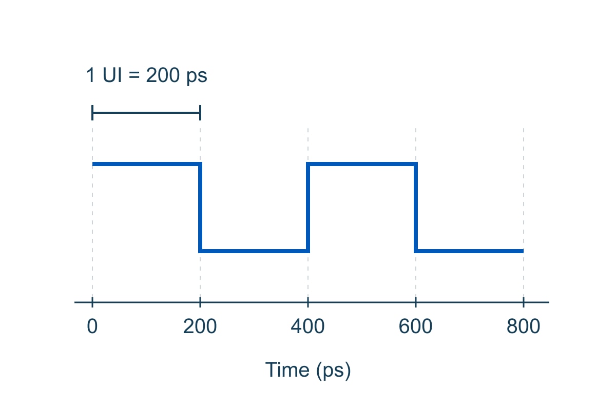
Input Where to obtain it Why it changes the answer
Finished trace width and copper thickness, mm Fabricator’s impedance proposal or approved stackup Finished geometry differs from a nominal copper weight or artwork width
Pair spacing and both side-ground clearances, mm Final copper or fabrication artwork; confirm edge-to-edge convention Pair coupling and side-ground coupling are separate effects
Dielectric height and Dk Approved stackup and material model Use the height to the actual reference and the appropriate dielectric value, not overall board thickness
Solder mask and local geometry Final mask artwork and solver model Coating and asymmetric copper can change what the simple cross-section represents

For the same pair, a plane on the next layer is not equivalent to a plane across the entire board thickness. Locate the actual signal and reference layer identifiers on the approved stackup. If the far-side plane is broken at the connector, mark that transition for separate review; a uniform 2D model does not evaluate the break.

Close view of two adjacent PCB traces and copper to their outside edges
Illustrative rendering. Verify the inner pair gap and the outer ground clearances independently in the final CAD artwork.

What to enter in a coplanar differential pair impedance calculator

Compare two calculators only after making their cross-sections and inputs equivalent. Start with the reference layers, finished dielectric height and copper thickness, then check Dk, mask, trace width, pair gap and outer gap. One tool may include mask or side copper in a way the other does not. Altium’s impedance documentation describes both the coplanar models and input differences that can explain disagreement.

Save an input sheet with units and a cross-section sketch, then change one parameter at a time in the same tool. This is more useful than averaging two outputs. If a calculator assumes symmetry but the real layout has ground much closer on one side, use a model that supports the actual geometry. At pads and layer changes, supplement the cross-section model with a suitable transition analysis or measurement.

Differential pair impedance formula

For a symmetric pair in odd-mode excitation, differential impedance is twice the odd-mode impedance of one line: Zdiff = 2 × Zodd. It is not necessarily twice the impedance of an isolated trace, because the neighboring signal and reference copper affect the fields.

For a teaching example, take a project target of 100 Ω ±10%, not a universal interface requirement. Its acceptance window is 90–110 Ω. If a symmetric model returns 48 Ω odd mode, the calculated differential impedance is 96 Ω. If a second model of the same pair with closer side copper returns 44 Ω odd mode, the result is 88 Ω. Those input values illustrate the decision and are not solver predictions for a specific geometry. The first result is in the window, the second is not; neither replaces a tolerance analysis or measurement.

Differential pair routing guidelines

Keep the final pair and its references consistent with the modeled profile. Repour copper and inspect the finished artwork before release: a ground island, neckdown, asymmetric clearance or plane split can appear after the initial routing check. Length matching does not make those cross-section changes disappear.

For the connector escape in the example, mark where the narrow fanout begins and ends. If the required ground clearance cannot be maintained there, review it as a local transition rather than applying a new trace width to the entire route. Check that adjacent copper is tied to the intended reference and that layer changes have an appropriate return path. Use the microstrip PCB guide for the underlying plane-referenced geometry.

What a PCB impedance test coupon can verify

A coupon is useful only when it represents the structure you intend to accept. For the coplanar route, ask the fabricator to identify the coupon’s stackup revision, signal layer, reference layers, pair spacing and side-ground arrangement. A coupon for ordinary differential microstrip can pass while saying nothing about a nearby-ground variant.

Check the impedance report against the fabrication drawing: match the coupon ID to the layer and geometry, confirm the target and tolerance, and identify the evaluated segment. If the report only shows “100 Ω pass” with no link to the modeled construction, request the coupon mapping and trace before accepting it as evidence for the coplanar pair.

Coax leads connected to a small PCB coupon on a laboratory bench
Illustrative rendering. A differential coupon result needs a known connection setup and an identified measurement region.

How to read a differential TDR measurement

A differential time-domain reflectometry (TDR) trace shows impedance changes along a path under differential stimulus. Agree on the fixture or launch reference, the part of the trace to evaluate and the pass window before comparing results. A connector discontinuity near the launch should not be mistaken for the steady region of a uniform coupon.

If the coupon is in range but the assembled link still fails, do not immediately change the straight-line width. Compare the actual launch, return path, layer changes and connector geometry with what the coupon omits. Use an appropriate link-level test for the required signal behavior. A passing coupon supports impedance control of the represented cross-section; it does not certify loss, mode conversion or the performance of the assembled channel.

FAQ

Can I leave a floating copper pour beside the pair?

Do not model a floating island as an ideal grounded reference. Inspect the final copper and its net connections. Remove the island or evaluate the actual structure if it must remain.
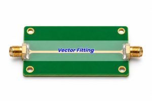
Does the quoted side gap include solder mask?

The gap normally refers to the copper geometry, while mask is a separate dielectric input. Confirm the tool’s drawing and the fabricator’s dimensional convention before comparing outputs.

Should I change pair spacing or side clearance first?

Start with the dimension the layout can actually change. Sweep it independently against the same stackup; if the result is too sensitive to production variation, choose a more tolerant geometry instead of optimizing only the nominal result.

Is an equal-length pair always symmetric?

No. Both traces can be the same length while seeing different pad shapes, nearby copper or plane openings. Check the surrounding geometry on both sides where the layout changes.

Can I use the same dimensions on a four-layer redesign?

Not without recalculating. The reference plane may be closer and the dielectric construction may differ even when the board thickness is unchanged. Get the new stackup and recheck the same routing profile.

Can a single-ended TDR reading be doubled to verify the pair?

Not if it is an ordinary single-ended reading rather than an odd-mode measurement. Use a differential setup or an explicitly valid mode conversion method and check how the instrument reports impedance.

Does every copper edge need a via fence?

No universal pitch or requirement applies. First decide whether the side copper is part of the controlled profile, then design its connection to the intended reference for the actual geometry and frequency range.
What files should I send for an impedance review?

Send the layer stackup, signal and reference layers, target with tolerance, relevant copper artwork, and the width and gap conventions. Highlight any local geometry that cannot follow the uniform cross-section.
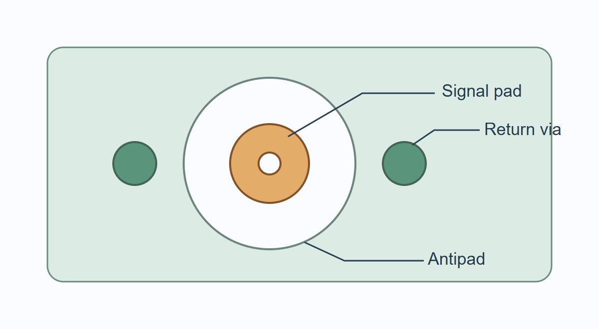
Technical references

For a Best Technology fabrication review, send the target impedance, stackup and routing cross-section to sales@bestpcbs.com.

You may also like

PCIe Backplane Guide: Map Lanes Before You Debug the Link
Friday, November 13th, 2026

A PCIe backplane connects one or more host links to devices such as NVMe drives. Start by tracing the lanes from the host to each bay. A connector can fit and a drive can power up even when the slot has no usable PCIe link. If the drive appears but runs below its expected width or speed, shift your attention from topology to the physical channel and link training.

Suppose a four-bay NVMe enclosure has a single x16 host connection. Four x4 drives are possible only if the hardware and firmware expose four usable links, or a PCIe switch creates four downstream ports. This guide follows that example from connector mapping to verification; it does not assume that every x16 slot can be split.

Server drive backplane beside a drive cage and NVMe trays
Map each bay to a host port or switch port before choosing the backplane. Illustrative rendering.

PCIe backplane board

The board is an interconnect assembly, not necessarily a controller. A passive version routes lanes, power and sideband signals; an active design may add switches, retimers or management logic. NVMe is a storage protocol that commonly runs over PCIe, while SAS and SATA use different interfaces. Physical bay fit alone does not identify what a given bay supports.

Draw a one-line block diagram showing host port, cable, backplane, bay and endpoint. Include any active device. If a product manual lists several backplane variants for one chassis, write down the actual assembly number and bay assignments before buying cables or drives.

PCIe backplane connector

Check the connector drawing and the host and backplane pin maps together. Verify lane order and direction, power, ground, reset, reference clock and any presence or management signals required by that platform. An identical housing can be wired differently; some cables are directional or intended for a specific host/backplane pair.

Parameter Record Acceptance evidence
Link width Host allocation and lanes to each bay Port map plus negotiated endpoint width
Link rate Gen4: 16 GT/s; Gen5: 32 GT/s per lane Agreed rate achieved under test; GT/s is not payload throughput
Channel pieces Host board, cable, backplane, drive interface Actual revisions in model and qualification record
Sidebands Clock mode, reset, detect and power sequencing Waveforms or system evidence under the agreed test plan
Service features Hot-plug, presence and LED ownership Verify only those features the product is designed to support
Close view of a server backplane connector bank and shielded cable
Match the actual connector and harness drawings; appearance does not establish the pin map. Illustrative rendering.

PCIe backplane chassis

The enclosure determines more than the board outline. Guide rails control how the drive meets the mating connector; cable bends and retention affect the harness; fans and blanking panels affect cooling around the drives and any active backplane devices. Two boards that mount in the same chassis may support different slots or protocols.

Dry-fit the actual cage and harness, then check every bay position with the intended carriers. Inspect alignment and cable strain, and record airflow and temperature in the populated configuration. A single drive on an open bench cannot verify a full chassis.

PCIe backplane riser

A riser typically changes where a link is presented; a backplane distributes connectivity across device positions. Some products combine both functions, so trace the schematic rather than relying on the name. Every extra connector or cable contributes its own discontinuities and loss.

If a drive works directly in the host but not through the installed riser, record the baseline negotiated link first. Add the riser and then the backplane or harness, one part at a time where the platform allows. Keep the drive, firmware and target rate unchanged so that the failing segment is meaningful.

PCIe bifurcation

Bifurcation divides a host link into separate links. A passive x16-to-four-x4 design needs the host port and firmware to support that specific split. An x8/x8 setting does not provide four x4 links. Check the platform’s port map and boot configuration before diagnosing missing drives as bad high-speed routing.

In the four-bay example, test a known-good drive in each bay individually, then populate all four. Compare the expected and enumerated ports. One visible drive and three invisible drives can indicate a topology or configuration issue; confirm this with the wiring and firmware evidence rather than treating the symptom as proof.

PCIe switch backplane

A switch provides separate downstream links while sharing upstream bandwidth. It can solve an endpoint-count problem when the host cannot offer the required split, but it adds power, cooling, configuration and recovery considerations. A retimer does not provide the same fan-out function.

Architecture Use when
Passive direct attach There is already one host link per endpoint and the channel meets its limits
Passive with host bifurcation The host supports the exact split and each link is routed to the intended bay
Switch-based fan-out You need more downstream ports and can accept shared upstream bandwidth and active-device overhead
Retimed link The topology is correct but the physical channel needs regeneration; port count stays unchanged

For the hypothetical enclosure, choose the switch version if the host exposes only one usable link and all four drives must enumerate. Then test simultaneous traffic; four visible drives do not guarantee four independent upstream bandwidth allocations.

PCIe 5.0 backplane

At 32 GT/s with NRZ signaling, the Nyquist frequency is 16 GHz. Use the relevant channel requirements and reference planes for the platform to evaluate the complete route, including cables, connectors, vias and boards. A 16 GHz loss number alone cannot capture reflections, crosstalk or frequency-dependent notches. A verified transmission-line geometry is only one part of the channel.

For a planning example only, assume 7 dB host routing, 9 dB harness, 5 dB backplane and 4 dB drive-side routing at 16 GHz. The simple sum is 25 dB before any connector or transition loss not already included. That is a bookkeeping screen, not a compliance result. Use cascaded channel data with consistent reference planes and verify the assembled link under the applicable tests.

PCIe retimer and redriver

A linear redriver uses analog equalization to compensate some signal loss. A retimer recovers the clock and data and transmits a regenerated signal; it participates in link behavior and creates separate electrical segments. Neither fixes an absent host port, incorrect pinout or missing power.

Check loss, reflections and topology first. If a redriver is a candidate, verify the whole link across its intended settings and variations. If you choose a retimer, validate each segment and the platform’s clocking, reset and training. In both cases, confirm the target rate and width across cold starts and load; one successful boot is not a release criterion.

FAQ

Why does only one NVMe drive appear?

First verify that the host provides the intended split or that the backplane has a working switch. Check bay mapping and use a known-good drive in each bay. Do not start by changing trace geometry.

Does a PCIe x16 connector mean all 16 lanes are wired?

No. The physical connector size and electrical allocation can differ. Check motherboard documentation and the link width actually negotiated by the installed device.

Can a SAS or SATA bay take an NVMe drive?

Only if that bay, controller path and cabling explicitly support NVMe. A shared form factor or matching connector housing does not establish protocol support.

Can a PCIe switch replace host bifurcation?

It can provide independent downstream links from one host link if the system supports the switch architecture. Verify enumeration, boot behavior, cooling and upstream bandwidth under simultaneous traffic.

Can a retimer fix drives missing because of bifurcation?

No. It conditions a routed link; it does not create more host or downstream ports. Confirm topology first, then check physical link quality.

Why does the same drive work at Gen4 but not Gen5?

The faster rate may expose channel margin, training or compatibility issues. Record the host, drive, cable and firmware versions. Compare with a known-good path and check the platform’s full channel requirements.

Is one successful boot enough for validation?

No. Check all bays, negotiated speed and width, errors under simultaneous load, repeat starts and recovery. Test hot-plug only on hardware designed for it.

What belongs in a backplane PCB review package?

Include the bay-to-port map, connector and cable part numbers, target width and rate, stackup, channel model and qualification plan. Keep chassis, firmware and drive revisions in the same record.

Technical references

Request a backplane PCB review

For a Best Technology PCB review, send the topology, stackup and relevant channel requirements to sales@bestpcbs.com.

You may also like