

PCB manufacturing PCB manufacturing
Home > Blog

Signal Integrity

LVDS Termination Resistor Guide: Value, Wiring and Layout
Tuesday, November 10th, 2026

Key Takeaways

  • A conventional point-to-point LVDS link usually uses one differential termination at the receiver, commonly 100 Ω.
  • The termination both develops the received differential voltage and reduces reflections by matching the transmission line.
  • A representative 3.5 mA current through 100 Ω produces 350 mV; these are nominal teaching values, not universal guaranteed specifications.
  • Internal termination can replace an external resistor only when the exact device, I/O bank and active configuration support it.
  • Two ideal 100 Ω loads in parallel produce 50 Ω. Whether two loads are correct depends on the topology.
  • AC coupling needs appropriate transmitter-side loading, receiver bias and signal behavior—not just two capacitors.
  • Approve the channel using the receiver waveform and timing requirements, not a resistance reading alone.

An LVDS termination resistor is a resistor connected across the two signal conductors at the receiving end of a typical LVDS link. A common value is 100 Ω, selected to match the differential transmission-line impedance and convert the driver’s steered current into a small voltage that the receiver can detect.

Getting it right involves more than selecting a 100 Ω part. The receiver may already contain termination, a connector may extend the electrical path, and AC-coupled or multipoint links need different arrangements. This guide explains the principles, calculations, connection options and PCB decisions so a schematic can become a testable design.
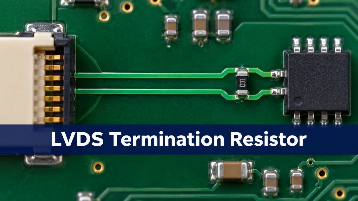
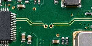
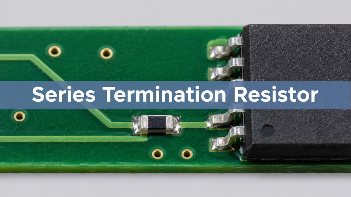
Circuit-board differential traces and a small part near a receiver package
Illustrative rendering, not a reference footprint or validated routing.

what is lvds

LVDS means low-voltage differential signaling: information is represented by the voltage difference between two conductors, rather than by either conductor’s voltage to ground alone. The receiver decides whether P is above or below N.

Define the differential voltage as Vdiff = VP − VN. The common-mode voltage is their average:

VCM=VP+VN2

A positive differential voltage does not require either pin to go negative relative to ground. In an illustrative 1.2 V common-mode system, P = 1.375 V and N = 1.025 V give +350 mV differential. Swapping these levels gives −350 mV. The two states span 700 mV differential peak-to-peak—not 350 mV peak-to-peak.

Consider a hypothetical data-acquisition board carrying ADC data to an FPGA. Each lane needs an electrically compatible receiver and a defined load; successful data capture also depends on clock-to-data timing. LVDS specifies electrical signaling, not the complete data protocol. See TI’s LVDS technology overview.

lvds termination resistor

In the usual DC-coupled point-to-point circuit, the resistor connects from P to N, directly across the receiver input pair. It is not inserted in series with either conductor and is not a pull-down to ground.

The driver steers current out along one conductor, through the load, and back along the other. Reversing the current direction reverses the differential voltage. The high-impedance receiver observes that voltage while the resistor provides the intended current path.

The same resistor is the load at the end of the transmission line. Matching the load to the line helps prevent an arriving edge from reflecting back along the pair. These are related functions: replacing the resistor with an open circuit removes the intended DC load and also creates a large impedance discontinuity.

For the ADC-to-FPGA example, trace the two nets all the way through adapters and connectors before drawing the termination symbol. A resistor already on a mezzanine card is still part of the circuit. Analog Devices explains receiver-end LVDS termination.

lvds termination resistor value

The familiar 100 Ω value follows from the intended differential line impedance and the driver’s operating load. It is a common starting point, not a resistor value to apply indiscriminately to every differential interface.

A nominal current-source model gives:

|Vdiff|≈IRT=3.5 mA×100 Ω=350 mV

TI’s LVDS Owner’s Manual uses this representative model. Actual guaranteed output levels come from the selected driver’s electrical table.

Parameter Value and scope
Differential termination 100 Ω; common design value
Steered current 3.5 mA; nominal model
Differential magnitude 350 mV typical; SN65LVDS1, 100 Ω
Specified output magnitude 247–454 mV; conditions below
Specified output common mode 1.125–1.375 V; SN65LVDS1
Nominal integrated load 110 Ω; SN65LVDT2 only

The SN65LVDS1 range above applies with RL = 100 Ω and 3 V ≤ VCC < 3.6 V under the datasheet’s specified conditions. At lower supply voltage, its minimum differs. The typical value is not a guaranteed minimum, and the nominal 1.2 V teaching example is not a universal input requirement. See the Rev M electrical tables.

lvds impedance matching

Match the termination to the pair’s differential characteristic impedance—not to the resistance of the copper traces. Characteristic impedance describes how a traveling wave relates voltage and current along the interconnect; a multimeter cannot measure it as a DC resistance.

For an ideal uniform line with real differential impedance Zdiff and a resistive termination RT, the load reflection coefficient is:

ΓL=RT−ZdiffRT+Zdiff

These calculations assume a 100 Ω line and an ideal 3.5 mA driver for the separate steady-state voltage estimate:

Load Load reflection Ideal settled magnitude
90 Ω −5.26% 315 mV
100 Ω 0% 350 mV
120 Ω +9.09% 420 mV
50 Ω −33.33% 175 mV

A positive coefficient means the reflected voltage has the same polarity as the incident wave; a negative value means opposite polarity. The percentage refers to the incident traveling voltage, not to bit-error rate or total signal loss. The settled-voltage estimate is not a prediction of the complete transition waveform.

A 120 Ω load can increase ideal settled amplitude while worsening the match to a 100 Ω line. That is why “more voltage” is not automatically better. Nonstandard values require both a device-load check and a channel assessment. The underlying reflection model is described in TI’s LVDS Application and Data Handbook.

lvds termination resistor power rating

Normal LVDS termination dissipation is small, but select the resistor using voltage across the load, not the IC supply voltage. For an ideal 350 mV differential magnitude across 100 Ω:

PR=Vdiff2RT=(0.350 V)2100 Ω=1.225 mW

Both polarities produce the same resistive dissipation. Using the 700 mV differential peak-to-peak value in this formula would overestimate the ideal two-state dissipation by four times.

A 1% external resistor is a practical starting choice when the design does not specify otherwise. Its package, temperature coefficient, rated-power derating and parasitic behavior still matter. A smaller package can simplify a short, symmetric connection, but assembly capability and inspection access also constrain the choice. Calculate margin from the actual maximum operating differential voltage and resistance limits; fault conditions need a separate review.

lvds termination resistor placement

Place an external termination close to the receiver input pins, with short and balanced connections to P and N. The electrical route from the resistor to the input matters more than the distance between component outlines.

If the resistor sits beside a connector but the receiver is farther inside the board, the segment beyond the resistor becomes an unterminated branch of the intended load point. It can still disturb the receiver even though the schematic shows a correct resistor value.

For scale, assume a 20 mm post-termination segment and a propagation delay of 6 ps/mm. Its one-way delay is 120 ps and its round-trip delay is 240 ps. Against a hypothetical 500 ps edge, that is not automatically negligible. These are teaching assumptions, not a universal length limit.

Place the resistor across the incoming pair without a long tee, an asymmetric detour or an avoidable via. A selectable footprint should remain compact even when unpopulated.

lvds internal termination

Internal termination replaces the external load only when the selected receiver actually provides it in the intended operating state. “LVDS-capable input” does not by itself establish that termination is present or enabled.

For example, AMD’s DIFF_TERM documentation describes enabling built-in 100 Ω differential termination. Availability and valid conditions depend on the FPGA family, bank, I/O standard and supply requirements. Treat those conditions as part of the hardware design, not just a software detail.

Choice Trade-off
Internal load Near input; device, bank and settings matter
External resistor BOM controlled; placement and tolerance matter
Selectable Flexible; document the active option

On the ADC board, record the FPGA input standard, bank supply and active termination setting alongside the BOM population option. Check reset and configuration behavior if the ADC starts driving before the FPGA is ready. Do not infer powered internal resistance from an unpowered ohmmeter reading.

lvds double termination

A conventional single-receiver link is overterminated if an external load duplicates the intended internal load. For two ideal 100 Ω resistances at the same receiving point:

Req=100×100100+100 Ω=50 Ω

The ideal 3.5 mA model then gives 175 mV rather than 350 mV. A real driver may depart from that model, and separated loads introduce transmission-line effects. Reduced amplitude alone therefore suggests a loading problem; it does not prove one.

Establish the active receiver setting and populated components, restore the intended load, then compare measurements using the same pattern and probe setup. A different topology, such as M-LVDS, can intentionally require two terminations; “two resistors” is not a universal fault diagnosis.

lvds ac coupling termination

AC coupling blocks the transmitter’s DC common-mode voltage, allowing the receiver side to establish another bias level. It also changes the DC current paths, so it must be designed as a complete interface.

Review three things together:

  1. Transmitter operation: Does the driver need a DC differential load, and where is that path maintained after adding capacitors?
  2. Receiver bias: Is the input internally biased, or does it need an external common-mode network?
  3. Signal behavior: Can the clock or data tolerate startup charging and baseline movement during long intervals without transitions?

TI’s LMK00301 datasheet, AC-coupled differential operation shows arrangements that differ according to receiver termination and bias. Some maintain a driver-side DC load and accept the resulting swing reduction when a receiving load is also present. That is a designed network, not the accidental duplication discussed above.

DC-balanced data or a suitable continuous clock is easier to AC couple than an arbitrary static level. For the ADC example, consider idle patterns and clock stoppage as well as the normal stream. Do not copy a capacitor value without checking the longest transition-free interval, startup requirement and both devices’ input/output conditions.

lvds split termination

Split termination uses two resistors whose series sum provides the differential load. Two 50 Ω resistors connected from P through a midpoint to N present 100 Ω to an ideal differential signal.

The midpoint determines what else the circuit does. A capacitor from that midpoint to ground can provide a common-mode AC return. A prescribed bias network can establish a DC level in an appropriate AC-coupled implementation. A capacitor alone does not establish a DC bias because it is open at steady DC.

With equal 50 Ω resistors and identical common-mode movement on both lines, the resistors appear in parallel toward the midpoint: 25 Ω before the midpoint network. This differs from their 100 Ω differential series path. Mismatched parts or asymmetric routing can spoil that symmetry.

TI SLAA840 includes split-termination examples. Use them when the common-mode or bias requirement justifies the network; adding a midpoint capacitor is not a generic cure for poor differential routing.

lvds multidrop

One driver feeding several receivers is not the same as several devices taking turns driving a bus. Establish that distinction before deciding how many loads to fit.

Topology Load arrangement
Point-to-point LVDS One load at receiver
Single-source LVDS multidrop One far-end load; short taps
Multipoint M-LVDS Both bus ends; matched devices

In the single-source multidrop arrangement described by TI SLAA840, the driver is at one end and the load is at the farthest receiver. Intermediate receivers must not each add another parallel termination. Their capacitance and branch lengths still affect the waveform.

M-LVDS drivers are designed for the heavier loading associated with two bus-end terminations. Two 100 Ω end loads give a 50 Ω DC equivalent, but the distributed bus is not simply a point-to-point LVDS circuit with another resistor added. Use devices and a topology intended for that service. Analog Devices AN-1177 explains the distinction.

lvds pcb layout guidelines

Route the interconnect as a controlled electrical structure, preserving its geometry and reference environment through the entire path. A correct load cannot repair an inconsistent pair.

  • Impedance: derive trace width and gap from the proposed finished stackup, not another board’s nominal dimensions.
  • Reference planes: keep the intended reference continuous beneath the pair; review every layer change and return-path transition.
  • Symmetry: use comparable pad exits, vias, connector paths and protection on P and N.
  • Stubs: keep optional footprints and test connections compact. A long measurement branch becomes part of the circuit.
  • Timing: meet the device’s intra-pair and clock-to-data timing requirements without unnecessary tuning structures.

“100 Ω differential” does not mean any two individually 50 Ω routes will remain a 100 Ω pair when brought together. Coupling changes the result. Finished copper, dielectric height, pair spacing, solder mask and the nearby copper environment must agree with the impedance model.

For a concrete manufacturing handoff, see the Best Technology LVDS PCB routing example; its dimensions are an example, not a universal recipe.
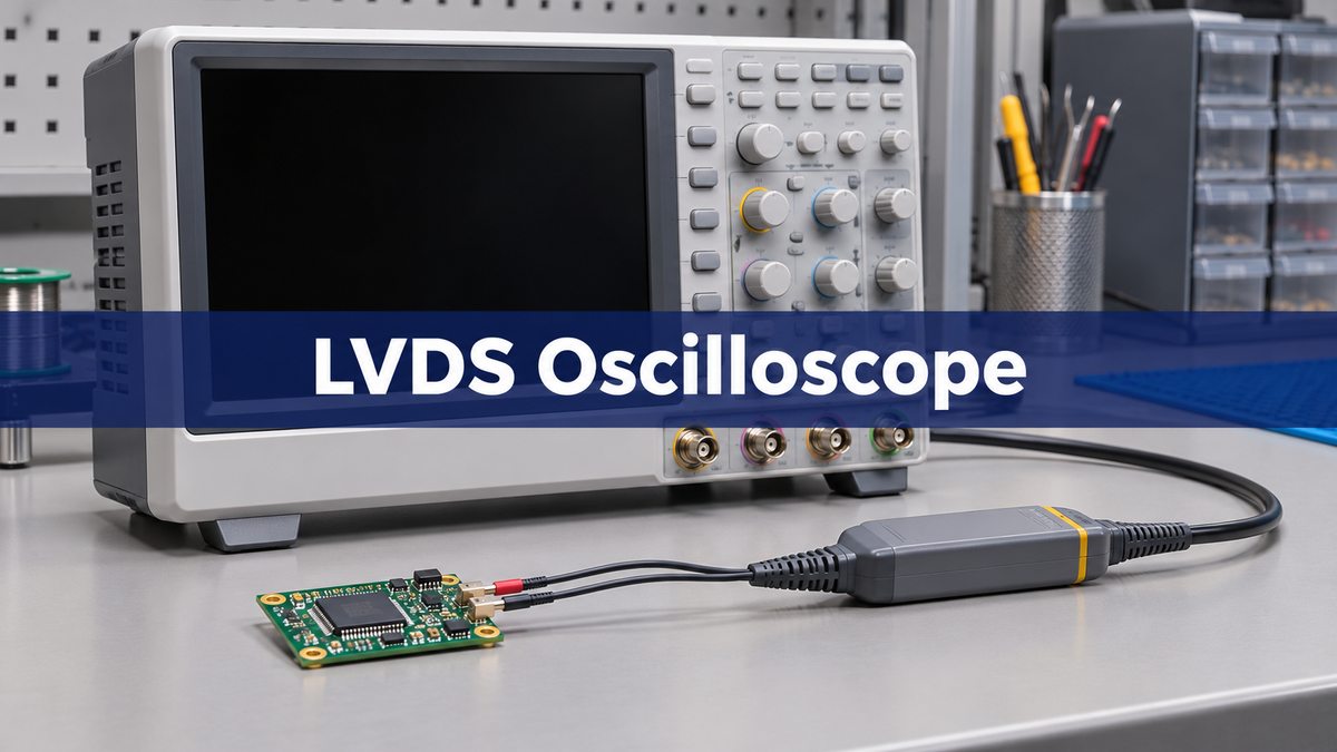
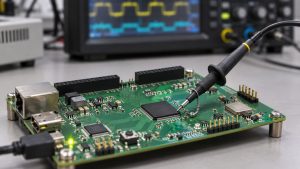
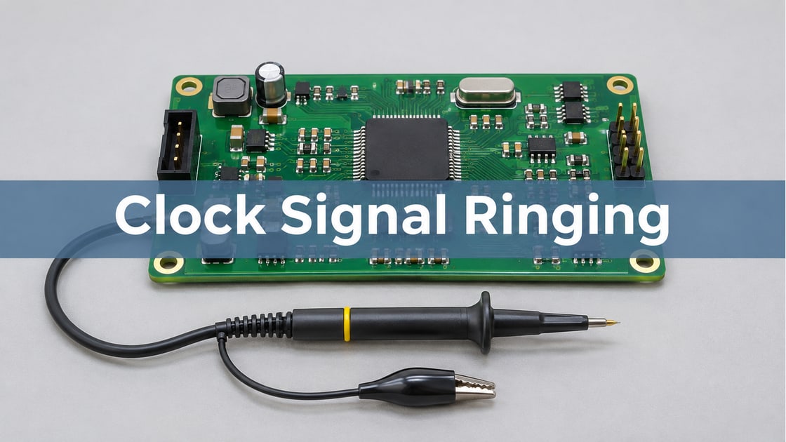
Oscilloscope and differential probe beside a small PCB
Illustrative rendering of a test bench, not a waveform or compliance result.

how to measure lvds signal on oscilloscope

Measure the differential signal at the receiver using a suitable low-loading differential probe, and examine both amplitude and timing. A clean waveform at the transmitter does not establish what arrives at the input.

  1. Record the data pattern, line rate, termination state, supply condition and probe point.
  2. Use bandwidth appropriate to the edge speed, and keep the probe connection short and symmetric.
  3. Measure differential magnitude, ringing and timing; assess common mode with an appropriate setup.
  4. Use an eye diagram and functional error testing where the interface requirements call for them.
  5. Compare results with the selected devices’ input limits and the project’s timing or eye criteria.

Do not attach ordinary grounded probe clips to the signal conductors. Nor should two 50 Ω-to-ground scope inputs be assumed harmless: they can introduce another 100 Ω differential load and alter common mode. Probing can create the fault you are trying to diagnose.

Power-off resistance measurements can identify accessible passive paths when the circuit allows it. They cannot establish characteristic impedance or prove powered internal termination. A TDR coupon checks representative fabricated geometry; the receiver measurement checks the operating channel.

lvds signal integrity

Signal integrity is the combined result of loading, interconnect geometry and timing—not a property established by one resistor reading. Before manufacturing, align the schematic, layout, assembly choices and receiver configuration.

For the hypothetical ADC-to-FPGA board, the release record should identify the exact endpoints, selected input standard, intended termination and population option, approved stackup, target impedance and tolerance, timing constraints, and verification plan.

Observed result Useful next investigation
Unexpectedly low amplitude Effective load and probe loading
Ringing near transitions Stubs, connectors and impedance steps
Good amplitude, capture errors Clock alignment, jitter and timing
Failure only at startup Bias, reset and configuration sequence

These are starting points, not diagnoses. Close the loop by testing the same board revision and operating conditions against defined pass criteria. If a load change improves amplitude but worsens the eye or error rate, the job is not finished.

Frequently Asked Questions

Can a 100 Ω termination make a 3.3 V transmitter compatible with a 1.8 V receiver?

Not by itself. Supply voltage and signal voltage are different quantities. Compatibility depends on differential swing, common-mode range, pin limits and the receiver’s bank rules. Termination does not replace a required level translator.

Can a short LVDS link omit the resistor?

Do not remove it just because the traces are short. A current-steering driver may still require the load to establish its output voltage. A termination-free implementation needs explicit support from the selected device documentation and validation.

Is LVDS a communication protocol like SPI?

No. LVDS describes electrical signaling. The interface still needs defined data organization, clocking and timing. Two devices can both use LVDS levels without exchanging compatible data.

Does an idle receiver automatically produce a known logic state?

No. Failsafe behavior depends on the device and the fault condition: open inputs, shorted inputs and an undriven terminated line are different cases. Select a receiver with the required behavior or use its recommended bias arrangement.

Should every unused receiver input get 100 Ω?

Not automatically. Follow the device’s unused-input instructions. A resistor across an unused input does not necessarily establish a valid logic state, while adding loads to connected bus taps can overterminate the bus.

Can an ordinary series resistor replace the parallel termination?

No. Series source termination is a different method. A resistor inserted in one or both conductors does not provide the receiving-end current path and load required by a conventional LVDS circuit.

Does a working clock prove that the data lanes are correct?

No. Each lane can have a different load, interconnect or timing relationship. Verify the affected lanes and their relationship to the sampling clock rather than approving the interface from one clock trace.

When is AC coupling the wrong starting point?

When the interface must convey a static state indefinitely, has uncontrolled long idle intervals, or lacks a defined bias and startup plan. Begin with the device-supported DC-coupled arrangement unless there is a specific reason to isolate common-mode levels.

Conclusion

For a conventional LVDS link, start with the intended differential impedance, one receiving-end load and compatible input conditions. Then make the resistor value, placement, internal configuration and PCB geometry describe the same circuit. For a Best Technology PCB fabrication discussion, send the stackup, controlled net list, impedance requirements and receiver-area routing to sales@bestpcbs.com. Bare-board manufacturing checks and complete-channel electrical validation serve different purposes; define both where the application requires them.

Technical References

You may also like

USB 2.0 Common Mode Choke: Check EMI and the Eye
Tuesday, November 10th, 2026

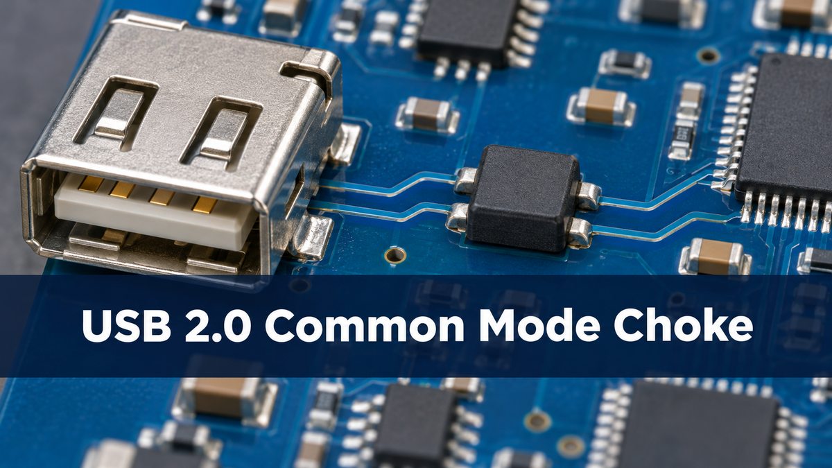
Add a USB 2.0 common mode choke only if the evidence points to noise on the data pair and the part improves emissions without consuming too much High-Speed signal margin. Compare a populated choke and a qualified bypass under the same test conditions. If emissions improve but the eye fails, the choke is not ready for production.

USB connector and a nearby small component on a circuit board
Illustrative rendering of a USB connector region, not a validated layout.

usb 2.0 common mode choke

A two-line choke uses coupled windings in series with D+ and D−. Ideally, signals flowing in opposite directions see little added impedance, while noise flowing in the same direction on both lines sees more. Real devices also have parasitics and differential loss. The part does not replace ESD protection, nor does it establish the pair’s PCB impedance.

usb common mode noise

First decide which path is carrying the noise. In a hypothetical USB service port, a radiated peak appears only when the cable is attached. That makes the cable a useful clue, not proof that D+ and D− are the source. Compare activity with controlled traffic and examine the shield and power paths. A data-pair choke will not necessarily address noise predominantly carried on VBUS or the shield.

common mode choke impedance

Read common-mode impedance versus frequency, then check the differential transmission and balance data. For example, Murata lists 90 Ω ±25% at 100 MHz for DLW21SN900SQ2 under its specified test conditions. That number is common-mode impedance at one frequency; it is not a differential routing target, bandwidth, or guarantee of attenuation in the product.

Parameter What to compare
Common-mode impedance, Ω Curve around the suspect frequency
Differential loss, dB Curve across the relevant signal band
DC resistance, Ω Maximum and balance between lines
Package and pinout Channel mapping and footprint

usb common mode choke selection

Prefer a device with relevant mixed-mode data and enough signal margin in the implemented layout. A higher catalog impedance at one frequency can still be the wrong choice if loss or imbalance increases. Keep a qualified bypass option where practical, but do not assume a jumper footprint is electrically invisible. Compare the routing geometry and inspect the built boards.

usb common mode choke placement

Follow the actual PHY and protection guidance. TI’s TUSB121x example places the choke close to the receptacle, on the PHY side of the ESD devices. That is a named implementation, not a universal placement rule. Preserve the shortest protection path from the connector and review the two parts together. See the USB 2.0 ESD placement guide for the separate transient-path check.
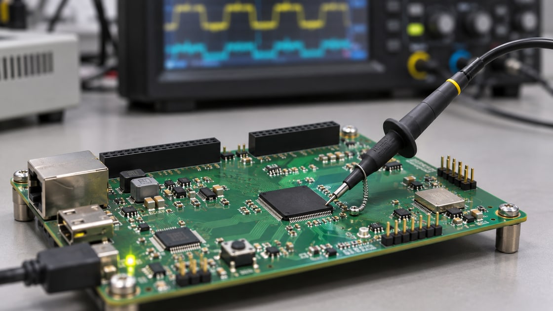
usb differential pair routing

Keep the pair symmetric through the connector, protector, choke pads and layer changes. If you provide bypass footprints, avoid an unused branch hanging from only one line. A common-mode problem can be aggravated by imbalance in the routing, so compare both the footprint and the continuous reference before asking the choke to hide a layout problem.
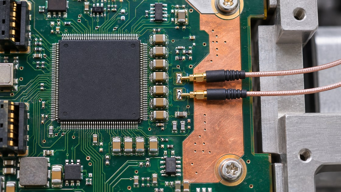
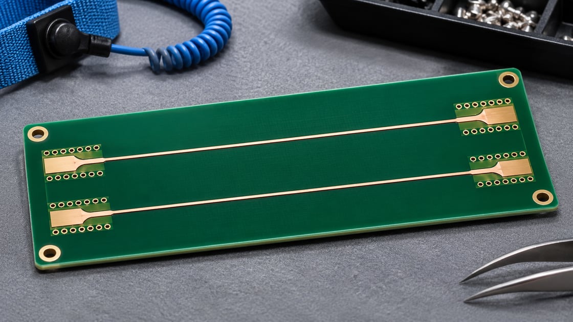
usb 2.0 radiated emissions

Compare the two builds using the same cable, orientation, equipment arrangement and representative activity. In the example, suppose the suspect peak falls by 4 dB after fitting the choke. That is an illustrative comparison, not a lab result or a compliance claim. Confirm the absolute result against the project’s applicable limit and check repeatability before crediting the component.

Outcome Decision
Emissions and eye both meet limits Confirm repeatability before release
Emissions improve but eye fails Reject; revisit part or routing
Eye passes but emissions do not improve Trace the actual noise path

usb 2.0 eye diagram

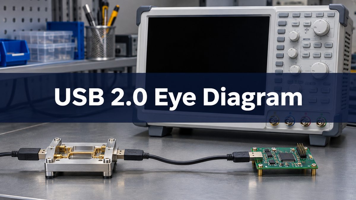
Verify the 480 Mbit/s High-Speed eye in the applicable test mode and fixture, not just enumeration or a short file transfer. A tight result with one cable is a reason to repeat the approved test under the required conditions, not to declare the change safe. For the controller example, release the choke only after the emissions result and the applicable USB electrical result both meet the agreed criteria.

USB test fixture and cable on a bench beside an oscilloscope
Illustrative rendering of a test bench. Use the specified USB test fixture and real capture for acceptance.

FAQ

Is the choke needed on every High-Speed port?

No. Use evidence from the intended system and the device guidance. A correctly working port need not add unnecessary loading.

Can I select a choke using only its 100 MHz impedance?

No. Compare frequency-dependent common-mode behavior, differential loss and the actual board measurements.

Can a bypass trial leave the pads empty?

Not if that opens the signal lines. Use the qualified bypass connection for the designed footprint.

Does enumeration show the High-Speed eye passes?

No. Enumeration is a functional observation. Use the applicable electrical test for the eye and signal limits.

Will the choke fix ESD resets?

Not by default. Inspect the discharge path and protection design separately, then verify the system’s ESD behavior.

Should I compare different cables in the first A/B test?

Keep the cable fixed for the first comparison. Test additional required cables separately to verify system robustness.

Can a data-pair choke fix VBUS noise?

Only if the coupling path involves the data pair and the change is shown to help. Inspect the power path if that is the dominant source.

Does a lower measured peak mean the product is compliant?

No. Check the applicable limit, modes and repeatability. A relative improvement and a compliance result are different claims.

Sources

TI TUSB121x board guidelines; TDK: USB 2.0 EMC practice; Murata DLW21SN specifications.

Project Review

For a Best Technology fabrication discussion, send the stackup, D+/D− geometry, connector footprint and choke or bypass options to sales@bestpcbs.com.

You may also like

CAN FD Termination Guide: Check Resistance and Ringing
Tuesday, November 10th, 2026

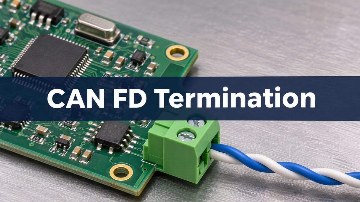
Start with two matched end terminations on a conventional linear CAN FD bus. With the bus safely de-energized and the applicable network isolated, about 60 Ω across CANH and CANL is a useful check for two nominal 120 Ω ends in parallel. It cannot tell you where those resistors are or whether a long stub is causing ringing. Check the physical ends next, then measure the differential and common-mode waveforms separately.

CAN controller PCB beside a twisted pair connected to a terminal block
Illustrative rendering of a CAN interface, not a validated circuit or a compliance result.

can fd termination

Termination matches the end of a transmission line to reduce reflected edges. The physical ends of the trunk are the ends that matter, not the two nodes with the lowest software addresses. Confirm the bus topology and cable impedance before applying the conventional two-end model. An engineered non-linear network needs its own analysis rather than extra resistors added by trial and error.

can bus termination resistor location

Walk the actual harness and mark both ends, every branch and any switchable termination. A termination at an intermediate node can still contribute the expected DC resistance while leaving a length of cable beyond it unterminated. In a hypothetical controller and sensor harness, a service node is plugged in midway and accidentally has termination enabled. If the far end is also missing its resistor, the meter can still show 60 Ω, yet the far end remains electrically open to an arriving edge.

can bus termination resistor value

For the conventional 120 Ω network, use a nominal 120 Ω differential termination at each physical end. In a split arrangement, two matched nominal 60 Ω resistors form one 120 Ω end. The midpoint capacitor adds a path for common-mode AC energy without adding a DC resistor across the pair.

Parameter What to verify
Nominal end resistance 120 Ω for the conventional cable
Split pair Two matched 60 Ω resistors per end
Midpoint capacitor Value, rating and return for this design
Resistor power Check fault voltage, duration and part rating

can bus termination resistance

With power removed and the network in the intended measurement state, compare the reading with the expected parallel combination. Two 120 Ω resistors give 60 Ω, one gives 120 Ω and three give 40 Ω in the ideal calculation. Treat those as clues, not acceptance limits: tolerances, other DC paths, internal switches and the connected harness can change the reading. Segment the harness as permitted and identify each termination before concluding that a board needs rework.

can fd split termination

Use a single resistor when the end is correctly matched and the common-mode behavior meets requirements. Consider split termination when the end match is right but common-mode disturbance remains an issue. It adds parts and a return path to review. It does not move a termination to the right place or shorten a stub.

Option Use when Verify
Single resistor End match and emissions are acceptable Value and physical location
Split pair plus capacitor Common-mode improvement is needed Matching, return and EMC result
Topology correction There is an incorrect end or long stub Reflection at the affected receiver

can bus split termination capacitor value

Choose the starting value from the transceiver and system guidance. NXP’s FS2400 example lists 4.7 nF as a nominal option, not a universal requirement. In a simplified common-mode model, the two 60 Ω branches act in parallel, so the effective resistance is 30 Ω. Together with 4.7 nF that gives about 1.13 MHz for the ideal RC corner. Cable and return impedances, parasitics and other components change the real response. That number is not a CAN FD data-rate limit and cannot predict compliance.

can bus signal reflections

If errors cluster after edges or at the faster data phase, look for timing and topology clues before changing the capacitor. On the hypothetical service harness, restore termination at the physical far end and disable the misplaced branch termination. Repeat the same capture. If ringing persists at one branch, compare the branch connection and length against the approved network design. A changing common-mode signal alone is not proof of a differential reflection.

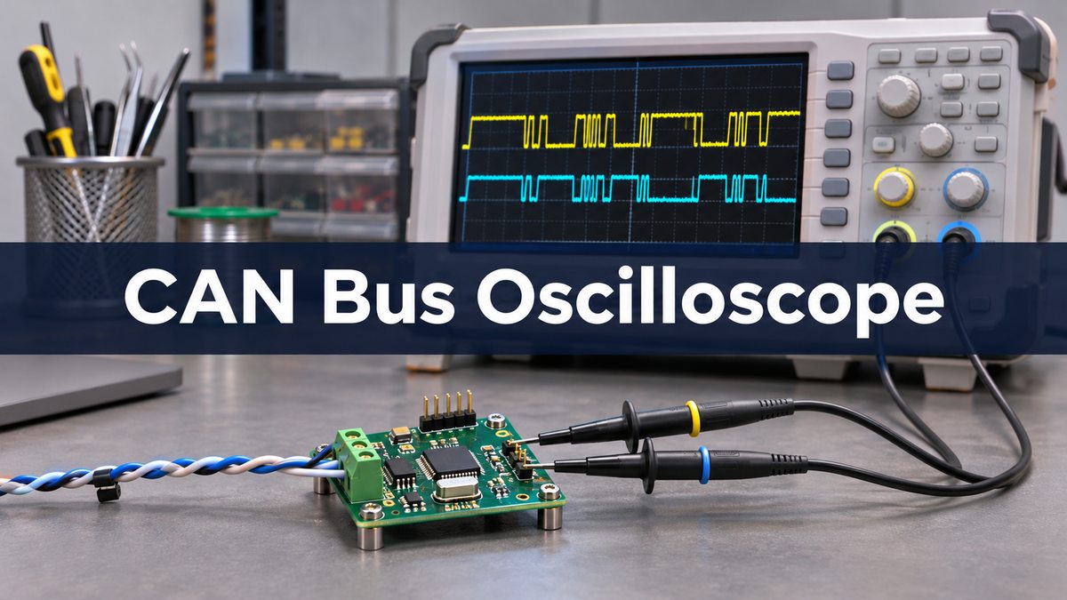
can bus oscilloscope waveform

Measure CANH minus CANL for differential behavior and, with a suitable referenced and matched setup, use their average to inspect common mode. Follow the instrument and equipment safety instructions and avoid grounding a floating bus through the probe. Compare the same receiver, harness, traffic and supply conditions before and after changes. Release only when the correct end map, resistance, waveform or timing limits, error behavior and any required system EMC tests meet the project plan.

CAN evaluation board and twisted pair on a bench near an oscilloscope
Illustrative rendering of a scope bench. Use calibrated measurements and the actual receiver location for comparison.

FAQ

Why do I see 60 Ω but still get errors?

The meter cannot locate the resistors or see stubs, receiver timing or interference. Confirm the end map, then capture signals at the failing receiver.

Should every node include an enabled 120 Ω resistor?

No. In a conventional linear trunk, enable termination at the two physical ends. An optional resistor footprint on an intermediate node can remain unpopulated or disabled.

Does split termination change the nominal differential DC resistance?

Not when each end still sums to the specified end resistance and the midpoint capacitor has no DC conduction path under the measurement conditions.

Can I choose capacitor size by looking at the data rate?

Not alone. The midpoint network targets common-mode behavior. Start from the device guidance and verify it against the actual noise and immunity requirements.

Does unplugging a node always leave the resistance unchanged?

No. The unplugged module may contain an end resistor or active termination. Identify what was removed and re-evaluate the expected reading for that configuration.

Should I fit a common-mode choke before changing the layout?

Check the failure mechanism first. A choke may help a specific emissions or immunity issue, but it will not correct an unterminated cable end or an overly long stub.

Is a clean waveform at the transmitting node enough?

No. Check the receiver that sees errors and other electrically distinct points. A reflection that is mild at one location may be significant at another.

What if the conventional 60 Ω rule does not fit this network?

Use the network designer’s topology and expected measurement state. Switched termination, active networks and branches require interpretation beyond the simple parallel model.

Sources

NXP AN14183: CAN components example; TI: TCAN evaluation module termination options; TI: split termination and common-mode behavior.

Project Review

For a PCB fabrication discussion, send Best Technology the board stackup, connector region and proposed termination footprints at sales@bestpcbs.com. If the protocol itself is still being selected, see the CAN bus vs LIN bus guide.

You may also like

USB 2.0 ESD Protection: Where to Put the Diode on a PCB
Tuesday, November 10th, 2026

For a USB 2.0 High-Speed port, start with a low-capacitance ESD diode close to the connector. Route D+ and D− past the protection pads without long branches, and give the diode a short return into the intended reference. Verify both USB signal quality and system ESD behavior: a board can enumerate and still reset during a discharge, or survive a strike and still fail the High-Speed eye test.

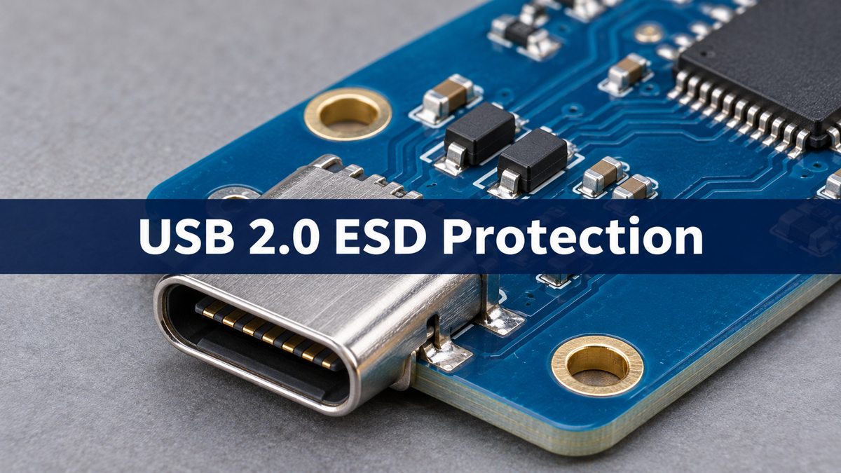
USB-C receptacle with small protection components at the edge of an assembled PCB
Illustrative rendering of a connector area, not a reference layout or a test result.

usb 2.0 esd protection

Protect the path from the exposed connector to the USB transceiver. When a transient exceeds the diode’s operating region, the diode conducts current into its return path instead of allowing all of the pulse to continue toward the transceiver. During normal signaling the device should remain off, but its capacitance still loads the pair. The goal is to minimize both the discharge loop and the disturbance seen by the data signals.

usb esd protection circuit

Draw two paths before choosing the footprint: the D+/D− signal path from the connector to the PHY, and the transient current path from each exposed data line through its protector into the designated return. The reference circuit for the selected part determines which pin is the return and whether the device uses a rail reference. A D+/D− protector does not establish protection for VBUS, CC or SuperSpeed pairs. For the rest of the interface, see the USB-C PCB design guide.

usb 2.0 esd protection diode

Choose a device against the PHY and connector requirements, not the largest advertised discharge rating. For example, TI’s USB application note lists ESD122 as a dual-channel D+/D− option with a 3.6 V reverse working voltage and 0.2 pF listed capacitance. Those figures belong to that device; use its current datasheet for test conditions and limits, then check actual layout and system behavior.

Parameter Decision check
Working voltage, V Check against normal line voltage
Line capacitance, pF Use stated test conditions and PHY budget
Clamping voltage, V Compare only at matching pulse conditions
Channel and package Confirm pin map and a routable return
Discharge rating, kV Check method; verify on the complete product

esd diode placement

Put the protector at the first practical point after the connector and keep both the connection to the data pads and the discharge return short. A component can look close in the placement view while its ground trace makes a long trip around a cutout. Check the copper layers and return vias, not just the component outline. Do not route the unprotected connector segment alongside sensitive circuitry if it can be avoided.

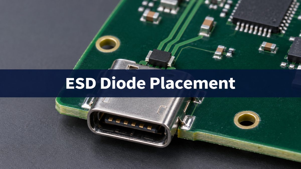
Close-up of a board-edge USB-C receptacle and a nearby black leadless component
Illustrative rendering. Verify the chosen footprint and discharge return on the actual PCB.

usb esd protection layout

Prefer flow-through routing when the part and footprint allow the data traces to pass directly through the protection-pad area. The diode remains a shunt element; the name describes the routing, not a series electrical connection. A short branch can be an alternative if the pinout forces it and the implemented design passes both signal and system ESD tests.

Routing option Use and trade-off
Flow-through First choice when pad map and return align
Very short branch Possible when constrained; measure the result
Long branch or remote clamp Revise: extra stub and transient loop

usb differential pair routing

Keep the two data paths physically similar through the connector, protector and first layer transition. Review reference continuity and avoid adding a long test stub to only one member of the pair. In a hypothetical compact service-port board that resets during cable-side testing, first inspect the discharge route and nearby reset or power circuits. If the same board also shows poor High-Speed signaling, check the diode capacitance, pad discontinuities and pair asymmetry before choosing a different clamp rating.

usb 2.0 differential impedance

The usual High-Speed differential routing target is 90 Ω nominal; confirm the tolerance and stackup requirements for the design. A calculated trace width covers the uniform section, not the pad and via transitions. Review those transitions separately, and include the protection device’s capacitance. The relevant data rate is 480 Mbit/s in High-Speed mode, but edge behavior is not determined by the bit rate alone.

usb 2.0 eye diagram

After a layout revision, verify the applicable High-Speed electrical test separately from the system ESD test. Use the specified USB test mode and fixture for the electrical test; for ESD, record the strike point, polarity, operating mode and allowed recovery behavior under the product test plan. Monitor real data traffic, resets and re-enumeration. Release only when the electrical result meets its applicable limits and the product meets its own ESD performance criterion. Successful charging or idle enumeration is not a substitute for either check.

FAQ

Can one array cover VBUS and the two data lines?

Some products can, but check the channel specifications and routing. VBUS operating voltage and exposure may differ from the data lines.

Is a larger TVS diode always a safer upgrade?

No. A larger part may add capacitance or create a worse return path. Check clamp behavior under comparable pulse conditions as well as link quality.

Can I place the protector on the bottom side?

Sometimes. Compare the complete path including signal vias, return vias and loop geometry. Verify the actual implementation rather than judging it by distance in a top view.

Should the common-mode choke go before the diode?

In TI’s TUSB121x example it follows the ESD protection. Confirm the sequence in the PHY and protector references and qualify it on the actual board.

Does a connector shield replace the data-line protector?

No. Shield bonding and signal-line protection address different paths. Follow the intended chassis and board grounding architecture rather than assuming they are interchangeable.

Why might the port restart even though no diode failed?

A transient can disturb the supply, reset path or reference. Capture the symptom and investigate the current route and nearby sensitive circuits before replacing the diode. The PCB ground bounce guide explains how a changing local reference can show up in a measurement.

Is a device-level rating proof of system compliance?

No. The assembled product adds connector, enclosure, layout and grounding variables. Verify it with the applicable system test and performance criteria.

Does this placement apply unchanged to USB SuperSpeed?

No. Check the separate transmit and receive paths, channel budget and AC coupling architecture. This guide addresses USB 2.0 D+ and D−.

Sources

Texas Instruments: ESD and Surge Protection for USB Interfaces; Texas Instruments: TUSB121x board guidelines; Nexperia: ESD protection for USB 2.0 interfaces.

Project Review

For a PCB fabrication discussion, send Best Technology the proposed stackup, pair geometry and connector-to-protector region at sales@bestpcbs.com.

You may also like

Source Series Termination: Diagnose Clock Ringing
Tuesday, November 10th, 2026

If a point-to-point SPI clock rings, check the signal at the receiving pin before changing the resistor. A second crossing of the receiver’s switching region is more important than how tidy the waveform looks at the driver. First rule out probe-induced ringing. Then compare the original board with a source resistor estimated from trace impedance minus effective driver impedance.

This guide follows one hypothetical 3.3 V clock from a controller to a single high-impedance peripheral. It explains what to measure, which resistor to try, and when the result is good enough to release. The numbers are examples, not measured performance or universal limits.

Close-up of a small series resistor beside a PCB output device
A series resistor placed near a PCB driver. Illustrative rendering; not a production record.

Source Series Termination

Source series termination puts a resistor between the output pin and the transmission line. The resistor and driver impedance together approximate the trace impedance. The first step travels to the receiver. At a nearly open load, the returning wave is absorbed at the matched source instead of repeatedly reflecting.

On an ideal 3.3 V rising edge with 50 Ω total source resistance and a 50 Ω line, the launched step is 1.65 V. The ideal open load doubles that incident step to 3.3 V. A real receiver has input capacitance and package parasitics, so the waveform will not exactly follow that example. A two-step waveform at the driver side of the line is not, by itself, proof that the receiver missed an edge.

Clock Signal Ringing

Measure at the receiving pin or the closest accessible pad. Use a short probe return and enough bandwidth to see the edge; keep the probe and acquisition settings fixed for each comparison. If apparent ringing changes substantially when you shorten the return, resolve the measurement artifact before tuning the board. Keep the capture time base wide enough to see settling and tight enough to distinguish closely spaced crossings.

Inspect rising and falling edges, not just the largest overshoot. Compare the excursions with the actual receiver’s datasheet voltage limits and input thresholds. If the waveform re-enters the undefined band, do not assume it clocked cleanly. Check transaction errors and, where available, compare the waveforms against receiver timing and hysteresis specifications.

Series Termination Resistor Calculation

Start with Rseries ≈ Z0 − Rdriver. For a nominal 50 Ω trace and a hypothetical effective 18 Ω output impedance, the estimate is 32 Ω; 33 Ω is a practical first build. Do not use the input pin impedance in place of driver impedance. Use an IBIS model or vendor data for a better estimate at the applicable voltage, drive setting and transition. Pull-up and pull-down impedances can differ.

Input Illustrative value What to verify
Trace impedance 50 Ω nominal Confirm routed geometry and stackup
Effective output impedance 18 Ω assumed Check IBIS or vendor data for both transitions
First resistor trial 33 Ω Compare against 0 Ω and adjacent values
One-way flight time 0.67 ns for 100 mm at 150 mm/ns Use the board’s actual propagation delay
Nominal round trip 1.33 ns Compare with measured edge and reflection spacing

Series Termination Resistor Placement

Route from the driver to the resistor first, then from the resistor into the controlled-impedance trace. Keep the driver-to-resistor segment short enough that it does not itself behave like a meaningful unterminated line for the edge in question. Do not leave a branch to an unpopulated alternate footprint or add a long measurement stub. Place any receiver test access where it can be probed without turning it into a branch.

For a board already fabricated, use the intended source resistor footprint if available. A component bodged near the receiver does not test source termination. Record the resistor package and placement along with the tested value so the result can be reproduced.

Bench probe checking a clock signal on a printed circuit board
Probe access at a PCB test point. Illustrative rendering; not a measured waveform.

PCB Trace Impedance

Use the actual edge time, not the clock’s repetition rate, to decide whether reflections matter. A modest-rate SPI clock can still have a fast transition. Obtain the line impedance from the actual fabrication stackup, with the trace referenced to a continuous plane. A split plane, poorly referenced layer transition or branch can produce a separate discontinuity that changing the source resistor cannot repair.

In the example, an apparent interval near 1.33 ns can justify inspecting a 100 mm path, but the estimate does not uniquely identify the reflection source. Check the actual route and compare both ends. If the measurement setup cannot resolve the expected interval, treat that as a limitation, not evidence of a clean edge.

Series Termination vs Parallel Termination

Choose the termination by load placement and drive budget. A clean point-to-point receiver waveform with small power cost often favors a source resistor. If the receiver-side termination needs to suppress the initial load reflection, a suitable parallel network can do so, but its DC or bias loading must be designed for the driver and logic levels.

Method Use it when Reason to change approach
Source series One driver feeds one high-impedance receiver at the end of a line Intermediate taps see a partial step or edge timing becomes marginal
Receiver-end parallel The far end needs a matched load and the driver can supply its current DC loading or bias compromises voltage margin or power
Topology correction first A branch, stub or broken return path dominates the waveform A resistor change does not remove the discontinuity

SPI Series Termination Resistor

Capture the baseline with 0 Ω, then try 22 Ω, 33 Ω and 47 Ω with the same cable, probe setup, drive strength and stackup. These are example trial values, not a mandated set. Inspect the receiver for excessive overshoot, undershoot, threshold re-entry and slow transitions. Also capture clock and data together, because a slower clock crossing changes setup and hold margins.

Release the smallest set of settings that passes on representative boards and under applicable voltage and temperature corners. Check both edge polarities, worst-case SPI activity, datasheet input limits and functional error rate. Document the test conditions and the chosen resistor. If all values fail, revisit measurement, topology, return path and driver slew before increasing resistance again.

Source Termination vs Load Termination

Probe both the receiver and, separately, the line side of the source resistor. A source match expects a return from the load; a load match is meant to absorb energy at the load. A two-step source waveform with a clean far-end transition can be consistent with source termination. Conversely, a visually clean source waveform does not prove adequate margin at the receiver.

Choose from the receiver’s actual failure mode. Keep source termination if the single end receiver passes voltage, switching and timing checks. Consider load termination only if its bias and current budget are acceptable. If the clock branches to several loads, model or measure each branch instead of carrying over a resistor chosen for a point-to-point design.

Frequently Asked Questions

Does a series resistor go near the clock source or near the receiver?

Place it near the driver for source termination. The resistor and output impedance must appear in series at the launch point of the line. A resistor near the receiver does not provide the same source match. A far-end parallel load is a different termination strategy.

Is 33 Ω always the right SPI clock series resistor?

No. It is a starting value for the example in this guide, where the line is 50 Ω and the output is assumed to be 18 Ω. A different stackup, drive strength, output impedance or receiver loading can make a different value work better.

Why did my clock work only when I touched it with a probe?

A probe can change the effective load, and its return can change the captured waveform. Treat the observation as a clue, not a fix. Repeat with a short return or lower-capacitance probe, inspect the layout and confirm that the circuit passes with the test equipment disconnected.

Can a low SPI clock frequency still cause ringing?

Yes. Reflections depend on the transition edge time and interconnect delay, not only on the clock frequency. Slowing the bit rate can help settle some signals between transitions, but it may not eliminate a receiver threshold re-crossing on a single fast edge.

Why does the source waveform show two steps?

The first step is set by the divider between the source resistance and the line impedance. A high-impedance load reflects the incident wave, which then returns to the source. Inspect the receiving pin to determine whether the receiver sees a single clean edge.

Will the same source resistor work with several SPI slaves?

Not necessarily. The inactive devices and branches can still load the clock line. Intermediate taps can see a partial step or branch reflection. Evaluate each receiving pin with its actual branch lengths and input loads, and consider changing the routing or adding buffering when appropriate.

Can too much series resistance create errors?

Yes. Excess resistance can slow the receiver transition or shift the time at which it crosses the switching region. Check setup and hold with the clock and data captured together. Do not choose a value solely because it gives the smallest overshoot at one test point.

What should I capture before approving the resistor value?

Record the receiver waveform for both polarities, the source-side waveform, the clock-to-data timing, voltage limits and representative transactions. Include drive settings, probe configuration and the board revision. Where the product requires it, repeat across supply and temperature limits before approving the value.

References

Discuss Your PCB Requirements

Preparing a controlled-impedance board for fabrication? Send the proposed stackup, target impedance and trace geometry to Best Technology at sales@bestpcbs.com. Include the layer transitions or connector locations that matter to your design review.

You may also like

PCB Ground Bounce: Isolate the Glitch Before a Respin
Monday, November 9th, 2026

When a quiet FPGA output glitches as neighboring outputs switch, repeat the capture with a shorter probe loop and change the number of switching outputs before changing the board. Then compare three voltages: quiet pin to local ground, local ground to receiver ground, and supply to its own local ground. These readings answer different questions.

Consider a hypothetical 3.3 V FPGA interface where an otherwise low status line appears to cross the receiver’s low-level limit when eight outputs switch. The oscilloscope trace alone cannot tell whether the receiver sees ground motion, a rail dip, ringing on one net or a probe artifact. Here is how to separate those causes and prove the fix.

Oscilloscope probe beside an FPGA development board on a lab bench
Use a short probing connection for a first check at the device. Illustrative rendering, not a production or test record.

what is ground bounce

Ground bounce is a transient change in voltage between two points treated as ground. When several outputs switch, their current may share part of the package and board return path. The voltage across that path can move even though both ends are on the same schematic net. A receiver responds to the signal relative to its own reference, not the zero line printed on an oscilloscope.

For the FPGA example, define driver-side board ground and receiver-side board ground before measuring. The die ground inside the package usually is not accessible. A board-level capture cannot measure it directly. A quiet output can serve as an indicator of switching noise, but it is not a direct reading of the internal ground node.

what causes ground bounce

A first-order inductive estimate is V = L × di/dt. If, hypothetically, 0.75 nH of effective common inductance carries a 0.16 A change in 0.8 ns, the estimate is 0.15 V. At the same current change over 1.6 ns, it is 0.075 V. These are sensitivity estimates, not measured peaks; actual current waveform, distribution, package and interconnect response matter.

The example explains why a lower repetition rate may not fix the glitch. Switching less often does not necessarily slow each edge. Change the number of outputs, programmed slew or load in controlled steps and measure what actually changed. The TI simultaneous-switching application report explains quiet-output test methods and why package and test conditions matter.

simultaneous switching noise

Keep the observed status pin low and use a repeatable trigger. Run the same pattern with one, four and eight outputs changing together; record direction, slew, drive strength, load, I/O bank, test points and terminations. Use the actual receiver or a known equivalent load. Compare both switching directions and capture multiple repetitions, not just a favorable screenshot.

Parameter Hypothetical comparison Control
I/O rail 3.3 V nominal Same receiver and rail setting
Aggressor count 1, 4 and 8 Same bank, load and switching edge
Quiet status pin Held low Same pin, node pair and trigger
Programmed slew Default then one approved slower setting Keep other settings fixed
Release limit Receiver input and system timing limits Evaluate measured waveform and functional errors

oscilloscope probe ground spring

A long ground clip can add loop inductance and pick up a nearby edge. Compare it with a ground spring on a suitable local return point, using the same probe, scope bandwidth and signal node where practical. A repeatable change with the probe arrangement is evidence of measurement sensitivity, not proof that the board has no problem. Document the geometry for any comparison.

Standard bench-scope ground clips are usually connected to protective earth and to one another. Do not clip them to nodes that must remain isolated, and do not defeat protective earth. For a ground-to-ground difference or a small differential voltage on a noisy common-mode level, use a suitable rated differential arrangement within its voltage, bandwidth and common-mode limits.

ground bounce measurements

Start with the status pin against the local return. Then use a differential measurement for the two ground points where practical, and measure the rail directly across nearby power and ground pads. If the issue is receiver behavior, also capture the signal at the receiver relative to receiver ground. Use comparable loading and bandwidth, then correlate the captures against the same switching event.

Node pair What it measures What it cannot establish alone
Status pin to driver-side ground Quiet output deviation near the driver Actual input waveform at the receiver
Driver ground to receiver ground Local board-reference movement Internal package ground motion
I/O supply to its local ground Local supply excursion Noise between two board ground points
Receiver pin to receiver ground Actual receiver input margin Which source created the excursion
Populated FPGA evaluation PCB with bench test leads near the logic device
Record the physical location and reference node for every capture. Illustrative rendering, not a production or test record.

simultaneous switching noise analysis

If the anomaly shrinks mainly when the probe loop changes, fix the setup and retest. If reference movement grows with output count and the receiver trace moves with it, investigate shared return and package/I/O choices. If the rail falls relative to its own return and the timing follows the rail disturbance, investigate the power delivery path. If one net rings while other measurements stay quiet, evaluate that net’s termination and discontinuities.

These are competing hypotheses, not mutually exclusive labels. Compare a known-good capture and change one variable at a time. Use the PCB power integrity guide when rail measurements point to a supply problem rather than a moving signal reference.

decoupling capacitor placement

Move or revise decoupling when the power-to-local-ground capture supports a supply-loop issue. A long neck or remote via pair can make a nearby-looking capacitor electrically far away at fast edges. Check the loop through package power, board vias, capacitor and reference return. Adding more capacitance does not bypass a broken return path and can change the PDN response.

If the rail is in budget and the receiver reference moves, compare a slower supported output setting or bank redistribution before changing the capacitor count. The trade-off is timing or pin-planning effort. A layout change to repair a shared return costs a new build but may be needed if configuration changes do not provide enough margin.

pcb ground plane rules

Trace the return path near the offending I/O bank and at every layer transition. Check the reference plane for voids or splits, nearby return vias, connectors and narrow ground necks. A layout correction cannot remove every package-internal effect; follow the device documentation for bank assignments and permitted switching conditions. See the via stitching guide for board return transitions.

Release the fix only when the worst approved switching pattern stays inside the receiver’s guaranteed input and timing limits with the agreed margin across required corners and no functional errors in the agreed test. Save the setup photo, revision, test nodes, I/O configuration, waveform and error counts. A cleaner screenshot at one temperature is not a release criterion.

FAQ

Can a long scope ground lead create a false ground-bounce trace?

Yes. A long loop can pick up nearby fields and produce ringing with the probe input. Recheck at the same signal point using a short local reference and a suitable probe. If the shape changes materially, record that effect before interpreting amplitude or using the original capture to justify a layout change.

Is ground bounce the same as supply droop?

No. Ground bounce compares reference points; supply droop is a drop in a rail relative to its own local ground. Both can occur during the same switching event. Measure both quantities separately and then confirm the voltage actually presented to the receiver rather than trying to infer it from a remote rail test point.

Why does the low output move if it never toggles?

A quiet low output can show switching noise because its output structure references a return path used by active outputs. That response may also include coupling or measurement artifacts. Keep the quiet output loaded as intended and compare how the disturbance changes with switching count, direction, probe setup and chosen reference.

Does slowing the clock eliminate ground bounce?

Not necessarily. A lower clock can reduce how often the event occurs, but each edge may still be fast and the same outputs may switch together. If the device permits it, compare output slew or switching alignment while checking timing. Keep the receiver load and trigger fixed for a meaningful comparison.

Should I add a larger decoupling capacitor first?

Not without rail evidence. A larger capacitor may help a slower supply excursion yet do little for a high-inductance local loop or a shared ground path. Measure across local power and ground, then evaluate placement, via geometry and impedance. Verify that a changed capacitor does not create another problem in the measured band.

Is ground bounce always worse on a two-layer PCB?

No. Package behavior, edge rate, load, stackup, routing and return geometry all matter. A second layer with a continuous usable reference can be better than several badly interrupted planes. Inspect the actual signal and return paths and confirm with a controlled measurement; layer count alone cannot qualify the interface.

Can I use two passive probes to measure between grounds?

Only with a safe setup and understood bandwidth, probe matching and common-mode error. Ordinary bench-scope ground clips are generally connected together through earth, so placing them on different nodes can disturb or short the circuit. Prefer a suitable rated differential method when that connection or accuracy is a concern.

What waveform proves the fix worked?

Measure the receiver pin against its own reference during the agreed worst-case switching pattern. Use device-specific guaranteed input levels and timing requirements, including the project’s required margin. Repeat at the necessary operating conditions and record functional errors, not just peak voltage; keep the probe setup fixed between baseline and revised captures.

Technical References

Request a Fabrication Review

For a Best Technology PCB stackup or layout review, send the board revision, return-path layout, I/O bank and switching pattern, probe reference points, and a failing and known-good capture. Include the receiver limits and the exact verification condition.

You may also like

PCB Trace Delay
Monday, November 9th, 2026

PCB propagation delay is the one-way time a signal takes to travel along a trace. For an initial estimate, multiply each trace segment’s length by its delay per unit length. Do not use one FR-4 constant for every layer: an outer-layer microstrip and an inner-layer stripline can have different delay rates even when their physical lengths match.

Suppose two signals must reach a receiver within a tight timing window. Equal lengths can look good in the PCB editor while the actual paths have different electrical delays. The useful comparison is in picoseconds at agreed reference planes, not just millimeters.

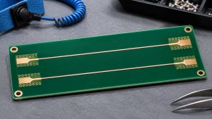
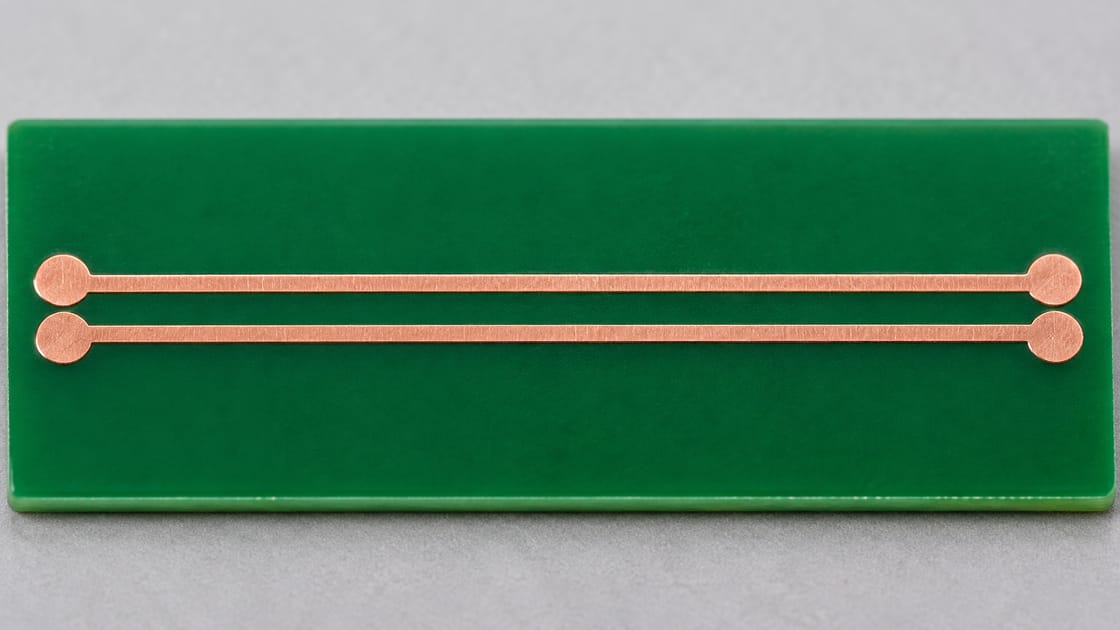
Bare PCB coupon with straight copper test traces
Each routing structure needs its own delay estimate. AI-generated illustration; not a coupon design.

pcb propagation delay formula

For a uniform, low-dispersion transmission line, estimate the one-way delay as t ≈ L√εeff/c. Here L is trace length, εeff is dimensionless effective relative permittivity, and c is about 299.792 mm/ns. The formula returns nanoseconds when length is in millimeters. For a route with several uniform structures, estimate each segment separately and sum the delays.

Input Unit Use
L mm Length of each segment
εeff None Line model
Speed of light mm/ns 299.792
Delay rate ps/mm Rate × L

Texas Instruments’ high-speed layout guide uses effective permittivity when comparing microstrip and stripline. Its example is a specific stackup, not an FR-4 rule. The approximation here also does not include connectors, package delay or a separate delay contribution from a via or launch.

pcb propagation delay per mm

In the simple model, the delay rate is about 3.336√εeff ps/mm. Multiply a ps/mm value by 25.4 to express it in ps/in. Compare the rates using the same units and without rounding too early, especially when converting a short timing budget into allowable length mismatch.

Model ps/mm ps/in
Microstrip (3.0) 5.78 146.75
Stripline (4.0) 6.67 169.45

At 80 mm, those two example lines take approximately 462.2 ps and 533.7 ps. Equal lengths leave about 71.5 ps difference before package and transition contributions. These are modeled values, not universal measurements or recommended limits. In a real board, use the stackup and trace model agreed for the applicable layer, not the example’s assumed values.

PCB test coupon and coax cables on a measurement bench
Define the measurement reference planes before comparing delay. AI-generated illustration; no measured results are shown.

fr4 pcb propagation delay

FR-4 is a material designation, not a single line velocity. A microstrip’s fields extend into more than one medium; laminate Dk, solder mask, trace width and height above the reference plane can all matter to the effective value. A homogeneous stripline approximation can use the surrounding dielectric value as a starting point, but mixed or asymmetric constructions still require a suitable model.

Microstrip vs. stripline for timing

When possible, route signals that must track each other through equivalent structures. If a layer change is unavoidable, ask for the relevant pressed thicknesses, material data and geometry so the solver can estimate delay by layer. Do not change to a different material solely to match the estimated velocity without also checking impedance, loss and manufacturing constraints.

pcb propagation delay calculator

Use a calculator only after choosing the units, reference planes and delay model. List every trace segment with its own delay rate; add a modeled or measured transition and package contribution if the timing budget includes those structures. Compare the complete path delays, not just their track-length totals.

  1. Decide whether the budget is for the bare board or the complete path to the device pins.
  2. Check the routing layers and divide mixed paths into uniform segments.
  3. Calculate with full precision, sum, then round the result for reporting.
  4. If the margin is small, confirm the model against a suitable coupon or measurement with agreed reference planes.

For a 50 mm outer segment at 5.7775 ps/mm and a 30 mm inner segment at 6.6713 ps/mm, the estimated trace-only delay is about 489.0 ps. Compare that with 462.2 ps for the 80 mm all-outer route: the same total length still leaves about 26.8 ps of difference. Add transition effects separately if the budget includes them.

A reflection on a TDR time axis includes travel out and back; that interval is not the one-way flight time used here. The TDR fault distance guide covers the separate round-trip conversion. Keep its time convention out of an end-to-end timing budget.

FAQ

Is propagation delay the same thing as impedance?

No. Impedance describes the voltage-to-current relationship of a traveling wave in the line; propagation delay describes travel time. A routing change can affect both, but matching nominal impedance alone does not guarantee equal delay. Evaluate each against its own requirement using the actual routing structure.

Should I use 150 ps/in for every FR-4 trace?

Use a rule of thumb for a quick feasibility screen, not as a final budget for every layer. A mask-covered outer trace and an inner trace can have different delay rates. Ask for a stackup-specific model when the difference matters to receiver timing or routing decisions.

Does equal PCB length guarantee that two signals arrive together?

Only if the paths have comparable delay per unit length and comparable contributions from transitions and packages. A board editor can report equal trace lengths for electrically different structures. Compare estimated time from the relevant launch to the relevant receiver plane before declaring the paths matched.

Do I include the device package delay in length tuning?

Include it when the timing requirement is defined at internal device reference points or when the component vendor specifies a package compensation model. If the budget is only for board connections, report package delay separately. Define the endpoint convention before adding package length or time to PCB results.

How does a via enter a propagation-delay budget?

Its effect is not always captured by adding the board thickness to the planar length. The transition includes a three-dimensional field and may add phase, loss and reflections. Use a suitable via model or measurement when the margin is small, and state whether the estimate includes that contribution.

Can a faster rise time change which delay estimate I should use?

A faster edge contains more high-frequency content. If the channel is dispersive, a single low-frequency delay may not describe the edge shape or timing of interest. Use an appropriate bandwidth and measurement definition rather than treating the simple low-dispersion model as exact at every frequency.

Should I measure a connector and trace together?

Measure them together if the requirement is for the complete interconnect. If you are trying to isolate the trace, use reference structures or agreed fixture removal to define the trace endpoints. Document which launch, cable or adapter contributions remain so another engineer can compare the results fairly.

How should I convert a skew budget into a length tolerance?

For two comparable uniform paths, divide the allowed time difference by the relevant delay per unit length. Do not use that shortcut across dissimilar structures without segment modeling. Apply package and transition allowances first if those contributions belong to the system’s budget.

Discuss Your Project

Send Best Technology the proposed stackup, routing layers, length or delay targets and timing reference points. Flag any planned layer changes or connector launches that need to be considered in the board review. Contact sales@bestpcbs.com.

You may also like

TDR Resolution
Monday, November 9th, 2026

TDR spatial resolution describes whether two nearby impedance changes can be distinguished, not simply whether a reflection can be detected. Compare their echo separation with the effective step response at the device. A sharp instrument specification or a fine cursor readout does not guarantee two usable peaks on a real PCB.

Consider a coupon with two small discontinuities a few millimeters apart. The practical question is whether the setup can report two locations, one combined event, or only a difference from a known reference.

Bare impedance coupon with a coaxial launch connector
The launch belongs to the measurement path. AI-generated illustration, not a tested coupon.

Separate detection from resolution

A time-domain reflectometer sends a step and observes reflections from impedance changes. One visible bump can indicate that something changed without showing how many features contributed. Resolving two features is the stronger claim: the trace must contain enough evidence to distinguish the two responses under the actual measurement conditions.

Record the parameters that set the test

Record time intervals, edge definition, velocity and reference plane before comparing plots. Distinguish the instrument’s specified step from the response available through the cable and launch. The resolution section of Tektronix’s TDR application note explains how step rise time, settling and ringing can cause nearby events to merge.

Parameter Record
Effective edge Rise time and threshold convention
Echo gap Interval on the reflection time axis
Velocity Measured or modeled path basis
Reference Calibration or fixture plane
Signal quality Noise, ringing and repeatability

Compare three different measurement claims

Choose the strongest conclusion supported by the data, not by the instrument’s display precision. A one-feature reference and a controlled two-feature coupon can help separate a real resolution result from a convenient interpretation of a broad trace.

Claim Evidence needed
An event exists Repeatable difference from reference
Two events resolve Distinct responses on matched setup
Feature sizes are known Suitable model and validation

Convert spacing to an echo interval

For two features on the same uniform line with one-way spacing d and propagation velocity v, their first-return spacing is approximately Δt = 2d ÷ v. Use d in mm and v in mm/ns to obtain ns. The formula describes expected timing, not a resolution specification. For absolute location or an instrument distance display, see the TDR fault distance guide.

Test the two-feature teaching example

Assume 3.2 mm spacing and 160 mm/ns velocity. The calculated echo gap is 0.040 ns, or 40 ps. A hypothetical effective 100 ps edge makes overlap a serious concern; a 30 ps edge is a better candidate for separation. Neither example is a pass criterion: amplitudes, polarity, ringing, fixture quality and noise still affect the result.

Treat rise-time rules as screening only

Published heuristics describe when small, similar discontinuities may be separated. Check whether a rule’s timing refers to one-way electrical separation, displayed reflection interval or a specific instrument convention before converting it to length. A known two-feature reference tested with the actual setup is a better basis for making a product-specific resolution claim.

Account for the path before the device

Cables, adapters and a launch can broaden the incident edge or add their own reflections. Document where the test plane is and what fixture treatment was used. If the suspected features are near a strong launch response, compare a reference with the same launch before treating a second shoulder as a separate defect.

Check the effect of polarity and magnitude

Similar reflections can merge into a broader feature, and opposite-polarity contributions can partially cancel. A small event next to a large one can disappear into its tail even when the spacing looks promising. Compare changes relative to an approved reference rather than counting visible peaks as a complete map of the underlying structures.

Coaxial cable and calibration terminations beside a PCB test coupon
Use a documented reference before interpreting nearby echoes. AI-generated illustration, not a calibration result.

Avoid confusing oversampling with bandwidth

A small sample interval can produce a smooth plot without recovering detail removed by a slow edge or bandwidth limit. Record acquisition settings, averaging and any filtering. Look for a stable conclusion when settings change within a controlled comparison; do not treat a software zoom or extra digits as a physical improvement.

Use an edge sweep as a diagnostic comparison

If the equipment supports controlled changes in effective edge, compare the same reference plane and coupon at two settings. A shoulder that becomes reproducible as the response improves deserves investigation. Changing the edge also changes how strongly some features appear, so use a reference and do not label the outcome as a universal acceptance threshold.

Validate a coupon against the intended question

For a fabrication test, confirm whether the deliverable is nominal impedance, a controlled discontinuity comparison or a resolution study. A routine coupon designed to measure a long uniform line may not answer the last question. Agree on feature spacing, construction, reference data and criteria before ordering a special verification coupon.

Report uncertainty instead of inventing a second location

State the feature geometry, timing basis, observed edge and what the trace supports. If two returns cannot be distinguished reliably, report a combined or unresolved event and identify the next check. The test can still narrow an investigation without claiming a defect count or location precision beyond the evidence.

FAQ

Does seeing one bump mean there is one defect?

No. A broad response can include multiple nearby discontinuities or a fixture contribution. Compare the expected physical features and a known reference before deciding what the event represents. If the setup cannot reliably distinguish candidates, report the observation as unresolved rather than assigning an exact count.

Can a TDR see a feature smaller than its quoted resolution?

A small feature may change the measured response relative to a suitable reference even when its two boundaries are not separately identifiable. Detection, separation and dimension extraction are different claims. State which one is supported by the evidence and avoid treating a visible difference as a calibrated feature size.

Does averaging make two reflections easier to separate?

Averaging can help with repeatability when noise is the limiting factor. It does not restore bandwidth or remove systematic ringing. Compare the same setup and keep the acquisition settings with the result. If two responses are still inseparable after noise improves, changing the edge or reference may be more useful.

Should I test at the fastest available edge?

Use an edge suited to the question. A fast setting can help identify nearby features, while a slower setting can help assess the response under a different relevant excitation. Record which setting supports each conclusion, and do not use one trace to imply performance at every system edge rate.

Can a VNA time-domain plot answer the same question?

It can support a related investigation if the frequency span, window, calibration and transform are appropriate. Its effective time response is not automatically identical to a direct-step TDR. Compare validated reference structures and report the settings and observable result rather than assuming the two displays are interchangeable.

Is a launch artifact always removed by calibration?

Not if the launch is outside the calibrated plane and remains part of the measured network. A suitable fixture treatment or a matched comparison may be needed. Record the physical plane and which structures remain included, then verify that a changed feature is not simply a different launch response.

Can the impedance coupon prove an assembled channel will pass?

No. The coupon can document behavior of its defined geometry under the measured conditions. An assembled channel includes connectors, components and other transitions, and can have different acceptance criteria. Use coupon evidence for the property it represents and perform appropriate channel verification separately.

What should a report say when separation is borderline?

Include the expected echo gap, effective response, test reference and comparison result. State whether the trace supports detection only or separation under specific conditions. If a decision depends on distinguishing the features, define the next controlled measurement instead of rounding the reported distance to imply greater certainty.

References and Question Research

Controlled-impedance inspection discussion informed the coupon and reference-plane questions; instrument guidance and the stated model support the technical explanation.

Discuss Your Project

For a fabrication or coupon review, send Best Technology the stackup, relevant geometry, test purpose and required evidence at sales@bestpcbs.com. Specify whether the request concerns nominal impedance or a separate two-feature measurement study.

You may also like

PCB Return Loss Guide: Read S11 Correctly
Saturday, November 7th, 2026

For an ordinary passive PCB interconnect, S11 displayed as log magnitude is usually negative, while return loss is conventionally reported as the corresponding positive number. S11 of −20 dB means 20 dB return loss and 1% reflected power at that frequency and reference plane. It does not mean 20 dB of forward signal loss.

This guide follows a hypothetical RF coupon between two coaxial launches. An engineer receives a plot and needs to determine whether it meets a specified reflection limit. The task is to read the quantity, sign, frequency range, and measurement boundary correctly—not to judge a PCB from one attractive marker value.

Illustrative RF PCB coupon with opposing coaxial edge launches
AI-generated physical-product illustration. No measured impedance or RF performance is represented.

What Does S11 Describe on a PCB?

S11 describes the reflected wave at port 1 relative to the incident wave at port 1 under the defined network conditions. It is a complex quantity, carrying magnitude and phase. The familiar negative-dB curve shows a transformation of its magnitude, not the complete complex result.

Keysight’s measurement-parameter documentation distinguishes reflection parameters S11 and S22 from transmission parameters S21 and S12. The port labels matter: a curve cannot be interpreted reliably without knowing where excitation and measurement occur and how the other ports are terminated.

Detailed S11 and Return-Loss Parameters

Write down the parameter definition before comparing a plot with a requirement. For equal real reference impedances in the usual passive interconnect context, use the following relationships. Here Γ denotes the input reflection coefficient and log means base 10.

  • S11 log magnitude: 20 log(|Γ|), in dB.
  • Return loss: −20 log(|Γ|), in dB.
  • Reflected power fraction: |Γ|² = 10−RL/10.
  • Record the reference impedance, frequency, calibration plane and termination conditions with every result.
S11 (dB) RL (dB) |Γ| Power back
−6 dB 6 dB 0.5012 25.12%
−10 dB 10 dB 0.3162 10%
−20 dB 20 dB 0.1000 1%
−30 dB 30 dB 0.03162 0.1%

These are calculated conversions, not PCB acceptance limits or measured results. The Teledyne LeCroy explanation of S-parameter terminology discusses the sign convention and the distinction between reflection and transmission.

Why More Negative S11 Means Less Reflection

A smaller reflected-to-incident wave ratio has a more negative logarithm. Therefore −30 dB S11 indicates less reflected power than −10 dB S11 at the same measurement conditions. Under the positive return-loss convention, the same comparison becomes 30 dB versus 10 dB.

Avoid saying only “lower return loss is better” or “higher S11 is better.” Name the plotted quantity. For our coupon, a specification of RL ≥20 dB corresponds to S11 log magnitude ≤−20 dB. These are the same reflection requirement written in two conventions, not competing performance targets.

Return Loss vs Insertion Loss

Return loss concerns reflected signal; insertion loss concerns reduction in forward transmission under the stated reference conditions. Their desirable directions differ. A positive return-loss value should usually be large, while a positive insertion-loss value should usually be small for a transparent interconnect.

Quantity Usual passive log-magnitude view What a transparent path aims for
S11 Negative dB reflection trace Small reflection magnitude
Return loss Positive counterpart of S11 log magnitude Larger positive value
S21 Forward transmission, often negative dB Near 0 dB within the intended band
Insertion loss Positive loss derived under stated conditions Smaller positive value

For the broader forward-loss question, see the RF PCB insertion-loss guide. Do not substitute that quantity for the reflection criterion.

A Worked Power Example for an RF Coupon

Suppose a hypothetical passive two-port coupon has S11 = −20 dB and S21 = −3 dB at one frequency, with equal real reference impedances and a matched output. The calculated reflected fraction is 10−20/10 = 0.01, or 1%. The forward transmitted fraction is 10−3/10 ≈0.5012, or 50.12%.

About 48.88% remains outside those reflected and transmitted terms in this example. Do not automatically call all of it dielectric heating: losses, radiation, unmodelled paths and measurement limitations need consideration. The lesson is that little reflection does not guarantee nearly complete forward transmission. This is a teaching calculation, not a test report.

Judge the Whole Required Frequency Band

A reflection limit applies over the specified band unless the requirement says otherwise. One deep S11 minimum can coexist with poor matching elsewhere. A marker placed at the best point cannot demonstrate compliance across an operating range.

For the coupon, record the band endpoints and the worst result within that interval. Under the positive return-loss convention, the weakest point is the smallest RL. Under the negative S11 log-magnitude convention, it is the point closest to 0 dB. Check the same band when comparing two revisions or suppliers.

Keep the Reference Impedance Attached to the Result

S11 is referenced to a defined port impedance. A result normalized to one reference cannot be compared casually with a different reference. The relevant value should come from the measurement setup, model, or supplied network data rather than an assumption based on connector appearance.

A nominally 50-ohm test system does not prove that every part of the physical coupon is 50 ohms. It defines a reference for evaluating the structure. If data are renormalized, record that transformation and its basis. Do not describe a changed reference as a physical improvement to the board.

Know Whether the Launches Are Inside the Measurement

The calibration and de-embedding boundary determines which structures the reported network includes. A measurement can contain cable adapters, connectors, launches and PCB traces, or represent a narrower region after an appropriate correction.

In our example, decide whether the requirement applies to the entire connectorized coupon or the trace region alone. Do not blame laminate properties from a launch-inclusive reflection result without further evidence. The related PCB fixture de-embedding guide explains the separate boundary question. A correction must be validated; it is not merely a cosmetic plot adjustment.

Illustrative RF coupon, coaxial cable and calibration accessories on a lab bench
AI-generated laboratory illustration, not an actual calibration or measurement record.

Why S11 and S22 Can Tell Different Stories

S11 looks into port 1; S22 looks into port 2. A structure with different launches or asymmetric discontinuities can present different reflection behavior from its two ends. Label the physical ports clearly before comparing curves.

Do not assume that similar forward and reverse transmission establishes identical input and output matching. In the controller’s RF path, the installed orientation can make the relevant end especially important. Record both reflection parameters when the test plan requires them and use the specified termination conditions rather than an undocumented open connector.

Single-Ended S11 Is Not Differential Return Loss

A differential interconnect needs the appropriate mixed-mode parameter and port definition. An individual single-ended S11 trace does not by itself describe the differential pair’s reflection behavior. Confirm the pairing, polarity and normalization used in the model or measurement.

Do not relabel a single-ended curve as SDD11 to match a requirement. Request the correct data or a documented conversion from a complete suitable multiport dataset. Keep the scope of this guide clear: the earlier numeric example is an ordinary single-ended two-port example, not a differential-channel qualification.

Investigate a Poor Result Without Guessing the Cause

Check the measurement configuration and repeatability before assigning a PCB defect. Verify connections, calibration applicability, port labels, data format, band and reference plane. Then compare the structure with its released design and any validated model.

A reflection feature can be associated with launches, geometry changes, vias, termination or other discontinuities. The S11 magnitude alone does not uniquely identify which one is responsible. Use additional evidence—such as a controlled comparison or an appropriate time-domain analysis—rather than announcing a root cause from the curve’s shape.

Report a Reflection Requirement Without Sign Ambiguity

A useful report names the quantity, inequality, band, reference impedance and measurement boundary. For example: “Calculated teaching requirement: return loss ≥20 dB across the stated band; equivalent S11 log magnitude ≤−20 dB.” Replace the example threshold with the actual approved requirement.

Include the dataset, setup notes and relevant uncertainty or validation limitations. For our coupon, release requires the agreed evidence across the band, not a universal “good S11” number. Keep forward transmission and other channel requirements in their own acceptance checks so one passing metric cannot conceal another failing one.

FAQ

Is −10 dB S11 better or worse than −20 dB?

For the ordinary passive reflection comparison at the same frequency and conditions, −20 dB indicates less reflection. It corresponds to 1% reflected power, versus 10% at −10 dB. Whether either result is acceptable depends on the actual requirement and operating band. Do not turn these conversion examples into universal PCB pass limits.

Why does a report call a negative trace return loss?

People sometimes use return loss informally to refer to an S11 log-magnitude plot. Read the axis, instrument format and stated formula before applying an inequality. If the report is ambiguous, ask the author to name the quantity explicitly. Changing a label without clarifying its definition can reverse an acceptance decision.

Does a 20 dB return loss mean 99% reaches the output?

No. It means 1% is reflected under the stated conditions. The remaining power is not necessarily all delivered through the intended output; dissipation, radiation or other paths may matter. Check the relevant transmission measurement separately. A well-matched attenuating structure is a useful reminder that input matching and forward transmission are different properties.

Can I add return-loss dB values along a channel?

Not as a general channel calculation. Reflections interact with phase and multiple discontinuities, so scalar return-loss numbers do not preserve enough information to predict the cascade. Use suitable complete network data and a validated connection model. Keep reference impedances, port orientation and measurement boundaries consistent when evaluating the combined structure.

Is dB the same as dBm on an RF plot?

No. A ratio expressed in dB is not an absolute power level in dBm. S11 log magnitude describes a wave ratio, while a receiver power readout can be an absolute quantity. Check the selected measurement and units before converting numbers or comparing them with a reflection specification. Similar-looking axes can represent different physical questions.

What if S11 appears above 0 dB?

First establish the device and measurement context. An active network is not covered by the simple passive assumptions used here. For an expected passive interconnect, examine calibration, processing, reference definitions and uncertainty before drawing conclusions. Do not merely flip the sign or delete inconvenient points to make the curve resemble a typical passive result.

Does a Smith chart contradict the negative-dB trace?

Not necessarily. A Smith chart displays complex reflection information in a different representation. A log-magnitude plot discards phase and shows only a magnitude transformation. Verify that both use the same frequency, port, reference impedance and dataset before comparing them. One view may reveal information that the other deliberately does not display.

What should a supplier send with a return-loss plot?

Request the measured structure identity and revision, port map, frequency range, reference impedance, calibration or de-embedding boundary, and the underlying data where available. Ask how the reported quantity and limit are defined. This makes the plot reviewable and prevents confusion between a connectorized coupon, a corrected trace model and a complete installed channel.

References and RF Enquiries

The linked Keysight and Teledyne LeCroy documentation supports the parameter definitions and sign conventions; the numerical examples are calculated and explicitly hypothetical. For a Best Technology RF PCB enquiry, send the stackup, geometry and measurement requirement to sales@bestpcbs.com. Specific fabrication and verification scope require confirmation.

You may also like

100-Ohm PCB Pair Guide: Are Two 50-Ohm Traces Enough?
Saturday, November 7th, 2026

Two traces that are each 50 Ω when modeled in isolation are not automatically a 100 Ω differential pair once placed close together. Mutual coupling changes the pair’s modal behavior. For a symmetric pair under differential excitation, the differential impedance is twice its odd-mode impedance—not necessarily twice the impedance of an isolated trace.

Two parallel exposed copper traces on a green PCB test structure
A pair of parallel copper traces. AI-generated illustration; geometry in a photograph does not establish impedance.

Follow a hypothetical interface whose specified differential target is 100 Ω. The designer initially selects a width that gives 50 Ω for one isolated trace, then places two such traces close together. We will distinguish what that calculation proves from what the actual pair still needs. The example does not assign a target or tolerance to every interface.

What Does a 100-Ohm Differential Target Describe?

It describes the transmission-line impedance associated with differential voltage and the corresponding loop current in the pair. It is not the DC resistance measured between the traces.

Each conductor has a voltage relative to the reference, while the receiver also sees the voltage difference between conductors. Those are different voltage definitions, so they produce different impedance definitions. AMD UG583’s transceiver guidance explicitly relates 50 Ω odd mode to 100 Ω differential. Its application-specific recommendation should not be copied as a requirement for an unrelated interface.

Which Impedance Parameters Must Stay Separate?

Name the excitation and current convention beside the impedance value. Otherwise, “50 ohms per trace” can refer to different calculations.

Quantity Meaning for a symmetric pair Example or relation
Isolated Z0 One trace without the coupled neighbor Assume 50 Ω
Odd-mode Zodd Per-line impedance under opposite excitation Assume 45 Ω after coupling
Differential Zdiff Between the pair under differential excitation 2 × Zodd = 90 Ω
Even-mode Zeven Per-line impedance under equal excitation Assume 60 Ω in that example
Common-mode Zcommon Common voltage divided by total pair current Zeven / 2 = 30 Ω

The numerical entries are illustrative model outputs, not results computed from the pictured board or a real stackup. The relationships follow the stated symmetric-line conventions.

Isolated-Trace vs Coupled-Pair Design

The isolated-line calculation omits the neighbor’s contribution, while the coupled-pair calculation includes it. Use the latter when checking the specified differential structure.

Design choice Useful check What not to assume
Choose width from isolated Z0 Single-line baseline Pair remains twice that value at every gap
Set width and gap together Actual coupled cross-section One width works on every stackup
Increase separation Recalculate both modes “Three widths” proves a target
Change layer or dielectric Re-solve the new structure Same artwork keeps the same impedance
Check a transition Use an appropriate transition model Uniform-line results cover pads and vias

This distinction concerns model scope. It is not a demand that every differential signal be routed with the tightest possible coupling.

Derive the Factor of Two from Voltage and Current

The factor of two comes from the differential voltage definition for a balanced odd-mode excitation. It does not require adding two physical resistors to the PCB.

Suppose one trace is at +0.5 V and the other at −0.5 V, with equal and opposite currents of magnitude 10 mA. Each trace’s odd-mode ratio is 0.5 V / 0.010 A = 50 Ω. The differential voltage is 1.0 V, and its loop current magnitude is still 10 mA, so Zdiff = 1.0 V / 0.010 A = 100 Ω. These assumed traveling-wave quantities explain the definition; they are not a DC measurement prescription.

A Worked Example Shows How Two Isolated 50-Ohm Traces Miss

If coupling changes the per-line odd-mode impedance, doubling the old isolated result no longer describes the pair. Recalculate the actual cross-section.

Assume an isolated-trace model gives Z0 = 50 Ω, but a separate coupled-pair model for the intended gap gives Zodd = 45 Ω. The pair is then 90 Ω differential, not 100 Ω. The 10 Ω difference is 10% of the hypothetical target; whether it is acceptable depends on the actual specification. The 45 Ω value is an assumed teaching output, not a prediction from width alone. No fixed correction factor converts every isolated 50 Ω design into the right pair.

Why Does the Gap Change Odd-Mode Impedance?

The adjacent conductor changes the electromagnetic fields and coupling between the lines. Opposite-polarity excitation is therefore not equivalent to removing the neighbor.

Polar Instruments AP157 distinguishes the odd, even and isolated modes. For ordinary symmetric edge-coupled structures, narrowing the gap generally lowers odd-mode impedance relative to the isolated case; widening the gap reduces the coupling. Check the actual cross-section rather than treating that trend as a numerical design formula. Nearby copper, dielectric boundaries and reference-plane geometry also belong in the model.

Solve Width and Stackup Together

Width, copper thickness, dielectric geometry and material properties influence the solution along with the gap. A gap adjustment should be assessed within the complete manufacturing construction.

For the hypothetical interface, ask the fabricator for the proposed cured stackup and achievable trace geometry, then solve the candidate pair using appropriate material data. Do not keep a width selected for a different layer height merely because its old calculation said 50 Ω. Record whether the dimensions describe artwork, finished top width or another geometry convention. A clearly named input is more reproducible than a screenshot of an unlabeled calculator result.

Can a Weakly Coupled Pair Still Be 100 Ohms?

Yes. In the weak-coupling limit, two equal lines approach independent behavior, and a pair of isolated 50 Ω lines can approach 100 Ω differential. Tight coupling is not the definition of differential signaling.

That limiting case does not remove the need for suitable references, balanced routing and interface-specific constraints. Evaluate whether the available routing geometry preserves the intended behavior along the path. A long uncoupled region, connector breakout and closely coupled region can each have different cross-sections. Avoid turning a general “route together” recommendation into an arbitrary universal gap requirement.

Even Mode Is Not Another Name for Differential Mode

Even-mode excitation drives the two lines with equal polarity, while odd mode uses opposite polarity. The same physical pair therefore has different modal quantities.

Using the assumed table value Zeven = 60 Ω, a common voltage of 0.6 V produces 10 mA on each line in the idealized mode. Total current is 20 mA, so the pair’s common-mode impedance under this convention is 30 Ω. This explains why Zeven and Zcommon differ by a factor of two. It does not prove that a real link has no common-mode noise or that an arbitrary termination is appropriate.

Bare PCB differential test coupon with two separate coaxial launches
Illustrative two-port coupon connection. AI-generated, not a validated launch geometry or impedance test record.

Recognize Where the Uniform-Line Model Stops

A two-dimensional cross-section describes a uniform line, not every pad, via, connector or reference transition on the route. Those discontinuities need an appropriate additional assessment.

Inspect where the teaching pair changes gap, enters a connector or moves layers. Do not infer that a correct straight-section result proves the entire channel meets its requirements. For relevant via geometry, the Best Technology differential-antipad guide addresses a separate design decision. Keep transition effects and line-target errors distinguishable so a local mismatch does not lead to unnecessary changes across the whole board.

Write the Fabrication Requirement in the Correct Mode

State the differential target, tolerance, layer, referenced structure and test expectations explicitly. Do not ask for “50 ohms on each trace” if the actual acceptance requirement is a differential pair.

A coupon and measurement plan should represent the intended construction within their agreed scope. Confirm the instrument’s mode and reporting convention before comparing values. A single-ended observation of one conductor is not automatically a differential result. The Best Technology differential-pair design guide covers the wider routing and manufacturing handoff; this article clarifies the impedance definitions within it.

Close the Design with a Reproducible Verification Basis

Retain the input construction, mode definitions, calculated result and agreed manufacturing evidence together. The objective is a controlled, verifiable pair—not a favorable number obtained by changing unnamed assumptions.

For the hypothetical link, verify that the final model satisfies its specified 100 Ω target and any other required channel criteria, then reconcile the production evidence with that basis. To discuss Best Technology fabrication requirements, send the stackup, routed layer, differential target and tolerance to sales@bestpcbs.com. Testing and modeling scope must be confirmed for the project rather than inferred from this educational example.

FAQ

Will a 100-ohm resistor make a 90-ohm pair become 100 ohms?

No. A termination sets the load seen at its location; it does not change the characteristic impedance of the distributed line geometry. Select termination according to the actual interface and analyze mismatches appropriately. Do not use a resistor substitution as evidence that an incorrectly modeled PCB cross-section now meets its fabrication target.

Why does my multimeter not read 100 ohms between the traces?

Characteristic impedance describes traveling-wave behavior, not simply DC resistance between two bare conductors. A multimeter can be affected by termination components or circuit paths, and an unconnected bare pair may appear open. Use an appropriate impedance measurement method and clearly identify the connected circuit before interpreting the reading.

Are all high-speed differential interfaces specified at 100 ohms?

No. Required impedance and tolerances depend on the interface and implementation guidance. The 100 Ω target in this article is a hypothetical teaching requirement, not a universal recommendation. Check the actual device and interface documentation before selecting geometry, termination or a fabrication acceptance limit for the project.

Can I double a single-ended TDR result to obtain differential impedance?

Not without establishing what the measurement represents. Exciting one line while treating its neighbor differently is not automatically a pure odd-mode measurement. Confirm the setup, terminations, calibration and conversion method. Doubling is valid for the defined odd-mode impedance, not every impedance trace displayed by a single-ended instrument.

Does correct differential impedance guarantee equal propagation delay?

No. Impedance and timing are separate design quantities. Geometry and materials influence both, but meeting one numerical target does not establish acceptable skew or total delay. Review the interface’s timing requirements and the actual path, including transitions, rather than treating an impedance pass as a complete channel qualification.

Does a symmetric drawing guarantee no mode conversion?

No. The manufactured structure, surrounding references, connectors and excitation can introduce imbalance even when two traces look symmetric in CAD. Maintain appropriate symmetry and analyze relevant discontinuities. A uniform-line impedance calculation is useful evidence for its own scope, but it is not proof that the assembled channel has zero conversion.

Can a solder-mask change affect the pair without changing its artwork?

It can alter the surrounding dielectric environment, particularly for outer-layer structures, so include the intended mask construction where it matters to the model. The size of any effect depends on the actual geometry and materials. Do not assume a fixed percentage change or approve a substitution without the relevant review.

Is impedance the only reason to keep a pair’s spacing consistent?

No. Consistent geometry also helps make coupling, propagation and the modeled structure predictable. Nevertheless, short constrained breakouts may require different spacing and a separate assessment. Apply the interface requirements and suitable analysis rather than forcing every segment into one gap at the expense of reference continuity or manufacturability.

You may also like