

Vector fitting turns sampled frequency responses into a rational model built from poles and residues. For PCB interconnects, that model can help a circuit simulator use measured or electromagnetic-extracted S-parameters in transient analysis. The important qualification is this: a smooth-looking fit is not automatically an accurate, passive or correctly connected simulation model.
Start with the complete complex data and a defined simulation task. Fit only after checking ports, reference impedance and frequency coverage; then validate the exported model, not just the fitting plot. This guide explains that workflow and provides an analytical one-pole example for checking units and numerical results. The example is synthetic, not a PCB measurement or a benchmark of any fitting package.
What is vector fitting?
Vector fitting approximates complex frequency data with a mathematical function that can be evaluated between samples and represented in a circuit-simulation workflow. It is useful when a measured or extracted interconnect is known by its terminal response rather than by a simple schematic.
A PCB trace, connector transition or package interconnect may be represented by an S-parameter matrix over frequency. A transient simulator still needs a numerical representation it can combine with drivers, receivers and terminations. A rational macromodel is one route; using the simulator’s direct S-parameter or convolution capability is another. Choose the route the target simulator supports and validate the result in that environment.
| Representation | Choose it for this job; check this limit |
| Sampled S-parameter file | Exchange terminal frequency-response data. The receiving simulator must define interpolation, extrapolation and time-domain handling; the file alone is not a complete driver/receiver model. |
| Vector-fitted rational model | Create a compact pole-residue representation for a supported simulation workflow. Check model order, residual error, physical constraints and export compatibility. |
| Known-topology equivalent circuit | Use when physically meaningful RLC or transmission-line elements capture the required behavior. Do not force an oversimplified topology to explain a complex multiport structure. |
For a short, simple interconnect, an adequate transmission-line model may be easier to inspect. For a complicated multiport response, a fitted model can be more practical. Neither option recovers missing measurement information or proves the structure behaves linearly at every drive level. Keep the characterization conditions with the model.
Vector fitting algorithm: what the iterations change
The algorithm relocates poles iteratively, then determines the residues and other selected terms for the resulting pole set. SINTEF’s algorithm description explains that the repeated subproblems are linear; this is more structured than drawing a smooth curve through magnitude points.
Think of poles as common dynamic features and residues as the contribution of each feature to an individual response. For a multiport network, sharing poles across responses provides one coordinated model rather than unrelated scalar curves. The residues can differ for S11, S21 and the other matrix entries.
Three choices still belong to the engineer: what data to include, how much model complexity to allow and which errors matter to the application. A numerical stopping condition says the algorithm stopped according to its rules. It does not say the input data are correct or that an omitted resonance has become irrelevant.
If a fit changes drastically when the initial settings change, investigate order, frequency sampling, noise and the data boundary. Preserve the original file and settings so you can compare runs. Do not repeatedly increase complexity until one plot looks convincing without knowing which result improved.
S parameter rational fit: prepare the complete complex input
Use the full complex responses required by the network model, with consistent port definitions and reference conditions. Fitting only S21 magnitude discards phase, reflections and coupling information that can matter when the model is connected to a real circuit.
Before fitting, identify each port’s physical location, signal/reference relationship, ordering and reference impedance. Confirm whether the data represent the bare trace, fixture-plus-trace or a de-embedded structure. A fitted model cannot correct a port swap that was never detected.
Record the frequency unit and range, number of samples, DC treatment and any preprocessing. Check both magnitude and phase for discontinuities or unexpected behavior. For detailed file interpretation, use the site’s Touchstone file guide; the fitting package should receive the same intended network, not a differently normalized or reordered version.
For a hypothetical four-port differential interconnect, prepare all 16 complex S-matrix entries at the defined frequency samples. Do not assume that fitting one through path establishes the other reflection and coupling paths. Whether symmetry or reciprocity can reduce independent information depends on the actual characterized structure and the model formulation.
Extrapolation needs separate attention. If the data begin above DC, the fitter does not magically know the DC behavior. If the target edge excites frequencies beyond the measured band, an in-band match does not establish the missing response. Obtain justified additional data or limit the model’s use; do not label extrapolated behavior as measured.
Poles and residues: read the model parameters
A common rational form is H(s) = d + s e + Σ rk/(s − pk), where s = σ + jω and ω = 2πf. The poles pk and residues rk describe frequency-dependent terms; d is constant and e is a proportional coefficient. The selected representation and simulator determine which terms are supported and appropriate.
The crucial unit distinction is between f in hertz and angular frequency ω in radians per second. Substituting f directly for ω moves the numerical corner by a factor of 2π. For a real-valued time response, complex terms must be handled with the required conjugate structure. Check the package’s representation instead of manually deleting a conjugate term because its plot seems redundant.
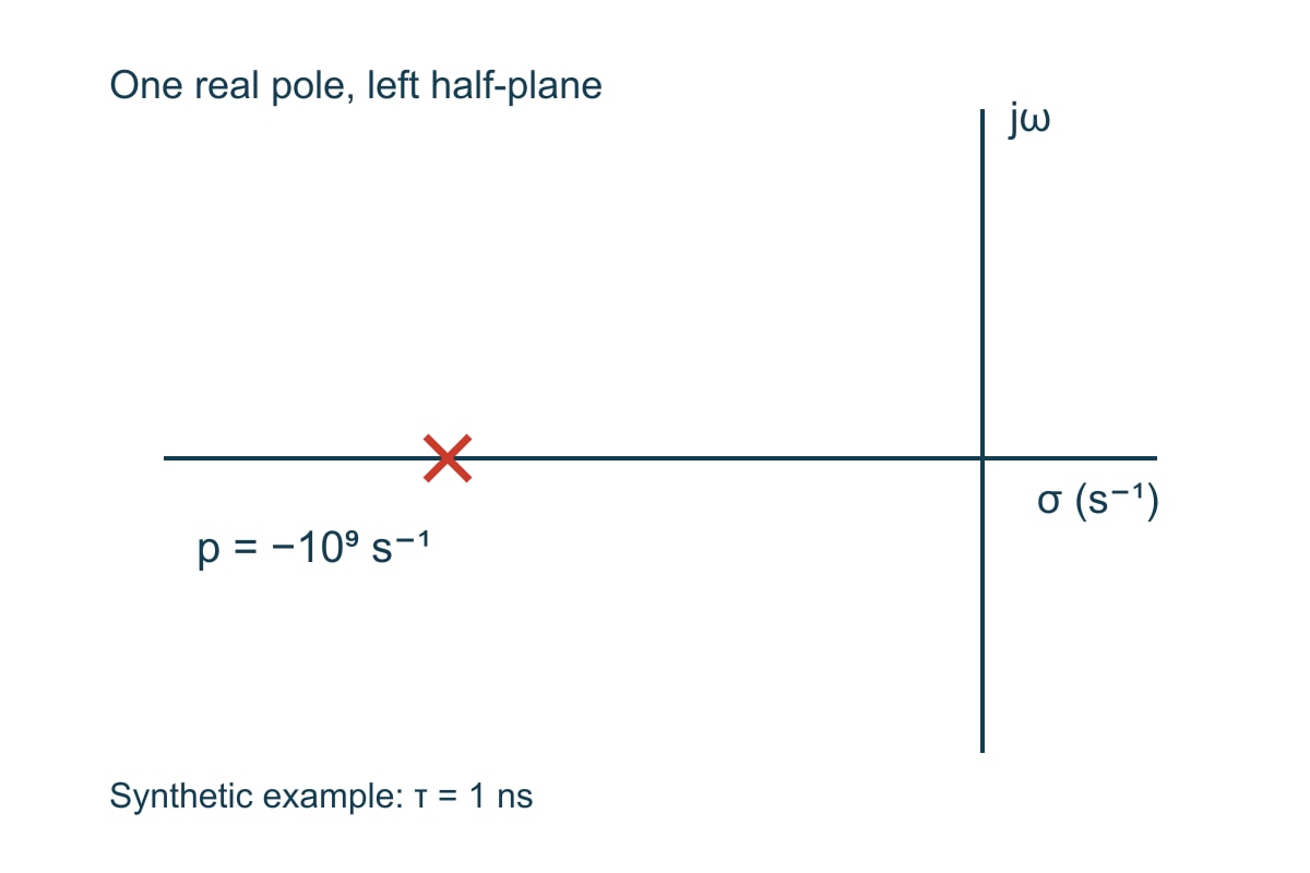
Here is a deliberately simple synthetic function: H(s) = 1/(1 + sτ) with τ = 1 ns. It is equivalent to H(s) = 10⁹/(s + 10⁹). The pole is p = −10⁹ s⁻¹, the residue is r = 10⁹ s⁻¹ and d = e = 0. This is a test function for learning and validation, not an extracted PCB channel.
| Quantity in this example | Value and meaning |
| Time constant τ | 1 ns; explicitly chosen teaching input. |
| Pole and residue | p = −10⁹ s⁻¹ and r = 10⁹ s⁻¹; their ratio gives unit DC response for this function. |
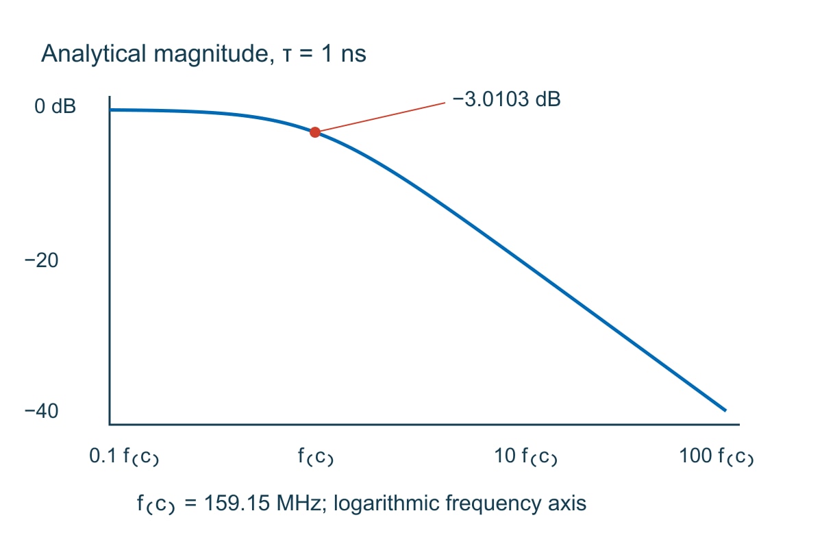
| Corner frequency fc | 1/(2πτ) = 159.154943 MHz, rounded to 159.15 MHz in the plotted label. |
| Magnitude and phase at fc | 1/√2 = 0.70710678, or −3.01030 dB, with −45° phase. |
| Magnitude at 10 fc | 1/√101 = 0.0995037, or −20.0432 dB. |
| Unit-step response at t = τ | 1 − exp(−1) = 0.63212056. This checks the same analytical function in the time domain. |
This example also shows why a pole’s numerical value is not its corner frequency in hertz: 10⁹ s⁻¹ corresponds here to 159.15 MHz, not 1 GHz. Compare any exported implementation against these analytical values before trusting the more complicated network workflow.
Model order: add complexity only when it improves the required result
Model order controls how much dynamic behavior the rational representation can describe. Too little order can miss structure; more order increases computation and can fit noise or poorly justified detail. There is no universal pole count for “a PCB model.”
Start from the response shape and the target application. Compare at least two reasonable settings using the same input data, weighting and evaluation frequencies. Inspect local residuals around resonances, reflections and low-amplitude coupling paths, not only a global average.
Use the one-pole function above as a controlled test: its analytical rational structure contains one real pole. Adding several poles should not be necessary to represent that exact noiseless function, although a numerical implementation may still return small numerical differences. If a simple test needs many modes to hide a unit error, increasing order is solving the wrong problem.
A long interconnect with substantial delay is different. Delay contributes phase that can demand a more complicated finite-order approximation over a wide band. Review the fitter’s documented delay handling or consider the simulator’s supported direct-data route. Do not claim that a higher pole count automatically makes the time-domain result more physical.
Passivity enforcement: recheck accuracy after changing the fit
Stable poles and passivity are different requirements. Stable poles concern the model’s internal dynamics; a passive network must not generate energy through its ports. SINTEF’s constraints discussion explicitly calls for a passivity check in S-, Y- and Z-parameter modeling rather than treating stable pole placement as sufficient.
For the intended passive interconnect, evaluate the complete fitted network with the applicable normalization and method. A satisfactory S21 magnitude alone cannot establish multiport passivity. The site’s S-parameter passivity guide covers that check in more detail.
The scikit-rf 2.1.0 passivity example demonstrates that a fit can look close to passive sampled data and still violate passivity. Its enforcement step also warns that the DC point cannot always be preserved. The engineering consequence is simple: enforcement is a model change. Compare its new complex responses, DC behavior and application result with the original requirements.
If enforcement needs large corrections, return to the input data, order and model assumptions. Do not repeatedly repair a model until the warning disappears while ignoring the response it now represents. An enforced model can satisfy a physical constraint and still be too inaccurate for the intended decision.
Vector fitting Python vs MATLAB: choose a usable delivery route
Choose an implementation by whether it can read your data, represent the required terms, test the relevant constraints and deliver a model accepted by the target simulator. A Python or MATLAB label does not establish accuracy or compatibility by itself.
scikit-rf provides documented vector-fitting functionality and examples in Python. SINTEF provides MATLAB-oriented implementations and documentation. Confirm the exact package version, dependencies, licensing and supported export path you intend to use; do not assume that every feature mentioned on a project website is present in every downloaded version.
A practical trial has three stages. First evaluate the analytical one-pole function to verify units and response interpretation. Next use a small representative network with known port mapping and compare the complex fitted data. Finally import the exported model into the actual simulator and check the same terminations and output quantities that matter to the project.
For a team handoff, deliver the input checksum or controlled revision, settings, software version, fitted model, validation record and port map together. A netlist without its reference impedance and port mapping may be syntactically valid but still be the wrong network. Compare the available signal integrity software workflows before choosing the model delivery route; verify the actual export in your receiving simulator.
RMS error and model validation: check the decision, not just the average
Use RMS error as one summary of residuals, then inspect where the error occurs and whether it changes the engineering result. A small matrix-wide value can hide an important local error in a weak coupling response or a narrow resonance. Define the error metric and weighting before setting an acceptance limit.
For a scalar response, one useful complex RMS definition is the square root of the mean of |Hfit − Hreference|² over the stated samples. That is not the same as RMS error in decibels or an RMS phase error. Record which definition the tool reports. Do not borrow a numerical “good fit” threshold from a demonstration and treat it as a release standard.
In a PCB channel application, preserve the through-path loss, phase and relevant reflections under the actual terminations; validate timing or eye results separately with appropriate endpoint models. In a coupled multiport application, check the weak paths and port coupling that determine the interference budget. In a passive filter model, resolve the transition and resonant features that set the filter decision. One average error cannot replace all three application checks.
Use this release worksheet after fitting and again after export. The first row demonstrates the numerical check. The remaining rows require project-specific inputs and criteria; they are not automatic pass/fail claims.
| Input or check | Expected decision and next action |
| Synthetic τ = 1 ns; evaluate at 159.154943 MHz | Reference magnitude 0.70710678 and phase −45°. A factor-of-2π frequency discrepancy means check hertz/angular-frequency conversion before fitting real data. |
| Port map, reference impedance and characterization boundary | Match the intended network. Resolve swaps, normalization changes or fixture inclusion before model approval. |
| Complex residuals across the required band | Compare local and summary errors with the application’s allocated tolerance. Missing out-of-band evidence limits the permitted use. |
| Pole structure and applicable physical constraints | Use documented checks for stability, realness and passivity where appropriate. Re-evaluate accuracy after any enforcement. |
| Exported model in the target simulator | Reproduce reference frequency responses and the required time-domain checks with the stated terminations. Import success alone is not validation. |
Vector Fitting S-Parameters FAQs
Can I fit an active device with vector fitting?
A rational approximation can represent active-device small-signal frequency responses, but do not enforce passive-interconnect behavior on an intentionally active model. Preserve the characterization conditions and understand what the linear model cannot represent, including nonlinear compression or a changing operating point.
Do I need to measure DC for every fit?
Not every task requires a measured DC point, but the low-frequency behavior must be justified for the intended simulation. Distinguish an added estimate from a measurement and check its effect on the time-domain result.
Why should phase be retained if I only care about insertion loss?
A transient network model needs the complex response. Different phase behavior can produce different delays and waveforms even when magnitude is similar. Fitting magnitude alone does not define the same causal dynamic model.
Does a lower RMS error always justify a higher-order model?
No. Determine whether the improvement occurs in the required responses and survives validation, rather than fitting noise or irrelevant samples. Compare runtime, constraints and the actual design result, not just one decreasing number.
Can vector fitting fix a wrong calibration plane?
No. It can approximate the response supplied to it, including fixture effects or calibration errors. Correct or explicitly include the characterization boundary before interpreting the model as a bare PCB structure.
Does passivity enforcement preserve all original data?
No. Enforcement changes the approximation and may alter DC or local response values. Recheck the changes against the error allocation and the intended simulation after enforcement and export.
How many responses are in a four-port S matrix?
There are 4 × 4 = 16 complex entries at each frequency. Physical symmetry or reciprocity can relate entries in an applicable structure, but the port map and model still need to preserve the required network behavior.
Does a fitted channel prove the fabricated PCB meets its specification?
No. A model represents particular input data and assumptions. Fabrication acceptance requires the agreed drawing, stackup, test conditions and evidence from the relevant produced boards or coupons. Simulation does not replace that evidence.
Custom High-Speed PCBs with Engineering DFM Support
Ready to turn a validated interconnect design into hardware? EBest Circuit provides custom PCB manufacturing and engineering DFM support. Reviewing the released stackup, controlled-impedance structures and fabrication files together helps expose build assumptions before they become a mismatch between your model and the manufactured board.
Send your Gerber or ODB++ files, stackup, impedance requirements, quantity and target delivery to sales@bestpcbs.com. Include the required coupon and test-report details. Request a fabrication review and quotation with construction, acceptance evidence and any open technical items clearly identified.
Technical References
- SINTEF: Vector Fitting, overview of rational macromodeling and applications.
- SINTEF: Algorithm, pole relocation and shared-pole fitting.
- SINTEF: Constraints, stable poles and passivity as separate considerations.
- scikit-rf 2.1.0: Vector Fitting, mathematical model and parameters.
- scikit-rf 2.1.0: Passivity Evaluation and Enforcement, example illustrating the need to recheck the fitted model.
You may also like







Tags: PCB Simulation, S-parameters, Signal Integrity, Vector Fitting