

PCB manufacturing PCB manufacturing
Home > Blog

S-parameter causality

S-Parameter Interpolation: Avoid False Insertion Loss
Tuesday, November 17th, 2026

Two S-parameter files can agree at every measured frequency and still predict different insertion loss between those frequencies. Before you call the PCB lossy, plot the original measured points over the solver trace. If the extra loss appears only between samples, check how the solver interpolated the complex data. In the worked example below, the interpolation mode alone introduces 3.01 dB of apparent extra loss. That is a calculated example, not a measured board result.
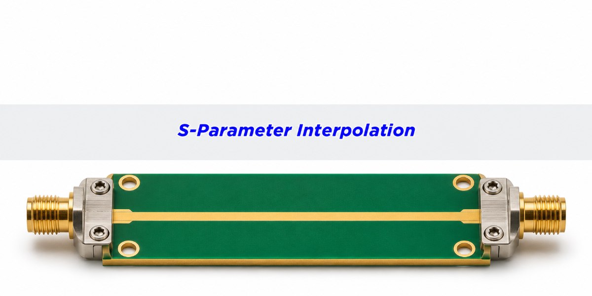
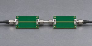
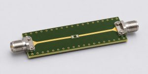
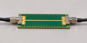
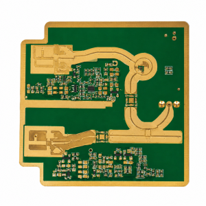
RF PCB transmission-line coupon with two coaxial launches and the S-Parameter Interpolation title
A two-port VNA sweep measures discrete points. A solver can generate more points, but it cannot measure what happened between them.

What Is S-Parameter Interpolation?

Interpolation estimates a complex S-parameter at a frequency between measured samples. For example, if the VNA recorded S21 at 4.00 and 4.10 GHz, the simulator may need an estimate at 4.05 GHz. S21 describes forward transmission under the file’s reference conditions; it has both magnitude and phase. A trace can therefore look smooth in dB while giving the wrong phase, or have the right phase but predict too much loss.

Keep the original export as the reference. Tag derived files as interpolated, and record the source sweep, target grid, method, port order and reference impedance. Treat guesses beyond the measured band, including a missing DC point, as extrapolation and review them separately. If your next step is to join two verified models, see this guide to cascading S-parameters with interface reflections before adding their losses.

What a Touchstone File Tells You About Interpolation

The Touchstone option line specifies frequency units and data representation. RI stores real and imaginary values; MA stores linear magnitude and angle; DB stores magnitude in dB and angle. These describe how the original points are encoded. They do not guarantee how the simulator fills in gaps. Re-exporting the same samples as RI does not, by itself, select Cartesian interpolation.

For a useful A/B comparison, keep the measured file, reference impedances, ports and target frequency grid fixed. Change only the interpolation setting. Compare both traces at the original points before investigating what they do between them. If they already differ at the original samples, check renormalization, reference-plane changes and any automatic fitting or smoothing.

Linear Interpolation Formula: Why the Midpoint Loses 3.01 dB

In this calculated example, a path has constant transmission magnitude of 0.800 and delay of 2.5 ns. Between 4.00 and 4.10 GHz its phase rotates 90°. At 4.05 GHz, polar interpolation yields −1.94 dB; Cartesian interpolation yields −4.95 dB. The PCB did not change. The latter method cut across the complex-plane arc.

Let t be the fractional position between the two frequencies. Cartesian interpolation computes (1 − t)S1 + tS2; polar interpolation applies the same weights separately to linear magnitude and unwrapped phase. Here t = 0.5, S1 = 0.800 + j0 and S2 = 0 − j0.800. The Cartesian midpoint is 0.400 − j0.400, with magnitude 0.566. The polar midpoint is 0.800∠−45°. Apply 20 log10|S21| to each magnitude to reproduce the numbers. Insertion loss, stated as a positive loss, is 1.94 dB versus 4.95 dB.
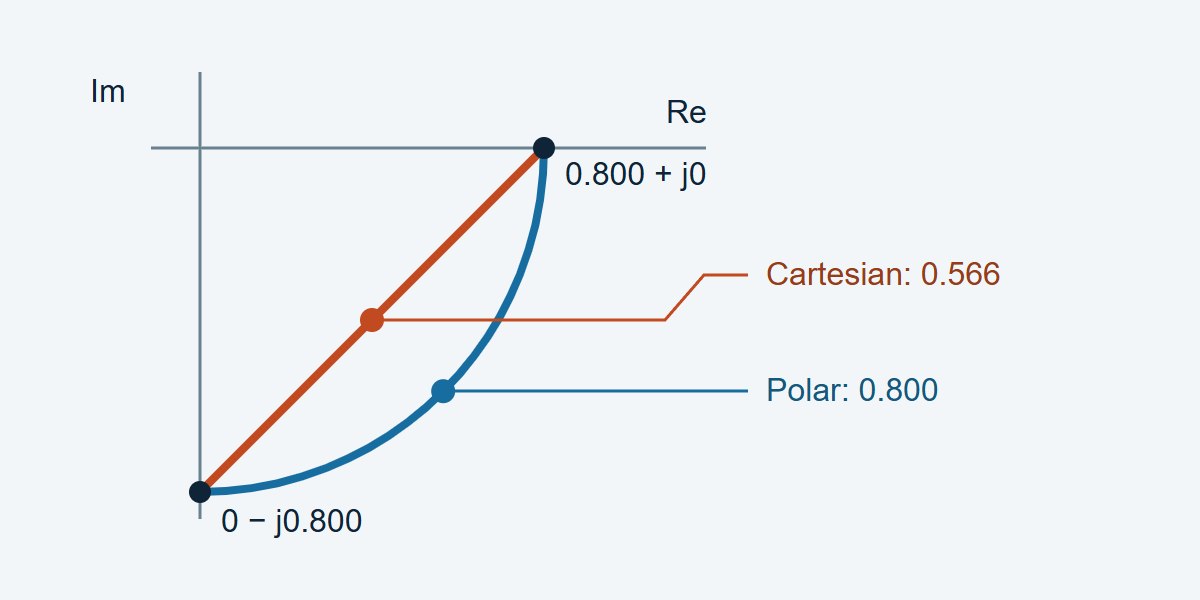
Complex-plane diagram comparing magnitude of 0.800 on the polar arc with 0.566 at the Cartesian chord midpoint
Same endpoints, different midpoints. The arc preserves magnitude in this idealized delay example; the chord does not.

Cartesian vs. Polar S-Parameter Interpolation: Which Should You Use?

Try polar interpolation for a smooth delay-dominated path and test it against measured points you did not give the model. Try Cartesian when the data pass near a null, where phase is difficult to interpret. If the raw sweep missed a narrow feature, neither method deserves a pass until a denser measurement resolves it.

S-parameter interpolation methods and the checks that decide between them
Method Try it when Watch for Verify with
Cartesian linear (real, imaginary) Phase becomes unreliable near a null; the complex trajectory is adequately sampled Chords create loss when phase rotates greatly per step Midpoint complex residual and S21 loss error
Polar linear (magnitude, phase) Transmission is smooth and delay dominates phase Phase unwrap can choose the wrong turn; phase near a null is unstable Measured phase trend, notch depth and ripple
Re-measure a finer sweep A notch, resonance or rapid phase rotation falls between samples Extra sweep time and drift between passes Convergence as spacing decreases, with unchanged calibration and fixture

Phase Unwrapping and Frequency Step Size

A 2.5 ns delay rotates the phase by 90° per 100 MHz, or 180° per 200 MHz. At 180°, a wrapped phase difference alone cannot tell the two directions apart. Even well below that figure, a Cartesian chord can still create unacceptable loss. Near a resonance or deep null, phase can change much faster than the nominal through-path delay suggests.

For a constant-amplitude, constant-delay path, the Cartesian midpoint amplitude ratio is cos(|Δφ|/2) when the actual phase step |Δφ| is below 180°. If the example’s Cartesian midpoint error budget is 0.10 dB, that model gives a maximum step of about 17.36° or 19.3 MHz at 2.5 ns. This is a starting sweep setting for the example, not a VNA specification. Check it with an offset sweep and tighten it where the DUT changes more quickly.

How to Check S-Parameter Interpolation Against Measured Points

Take a calibrated sweep on a fine grid. Save alternating measured points as a separate verification file, then feed only the retained points to each interpolation method. Compare the predicted results at the withheld points against the saved measurements. Keep VNA settings, fixture, reference planes and signal path unchanged. Repeat near critical frequencies if the measured trace is close to the acceptance limit.
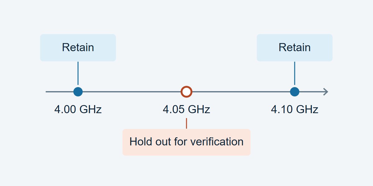
Holdout validation diagram showing retained 4.00 and 4.10 GHz points and the independent 4.05 GHz verification point
Do not give the 4.05 GHz verification value to the interpolator. Replotting a generated point on a denser display is not independent validation.
Holdout worksheet: what to enter, how to judge it, and what to do next
Check Record Decision and next step
Through loss at 4.05 GHz (example) Calculated reference −1.94 dB; Cartesian −4.95 dB; residual 3.01 dB Fails a hypothetical 0.10 dB budget. Try polar, then confirm against an actual held-out sample.
Delay-sensitive band Wrapped phase residual at each held-out point; group-delay residual if required If outside the design budget, verify phase unwrap and retest with a finer grid.
Filter notch or resonance Measured and predicted feature frequency, depth and critical-band residual If the fitted shape or frequency fails, measure locally at finer spacing. Near the noise floor, assess uncertainty before classifying depth errors.

S-Parameter Passivity Check After Interpolation

For a passive network, check passivity over the generated grid, not only at the original points. Where ports use fixed positive real references and power-wave normalization, the largest singular value of the full S-matrix must not exceed one for ideal passive data. An S21 magnitude below one does not prove the network is passive. Evaluate numerical or measurement tolerance separately from the ideal bound.

With a shared linear weight and identical normalizations, Cartesian interpolation of two passive whole matrices preserves the singular-value bound between them. That result does not carry over to arbitrary cubic interpolation, element-wise polar interpolation or causality. For impulse or step simulations, use the solver’s grid requirements and review the S-parameter causality and time-domain checks separately.

S-Parameter Simulation: What to Check Before You Release the File

Channel-loss budget: keep the full band needed for the channel model, identify the frequency or band where spec margin is tightest, and allocate an explicit dB error budget to interpolation. If the residual at an independent point exceeds that budget, do not use the dense model for sign-off.

RF filter model: check that the generated file preserves the passband ripple, stopband rejection and notch location at the frequencies in the filter specification. Add measured points near features rather than relying on a smooth trace or an interpolated null.

Time-domain use: log the measured band and any assumed DC or high-frequency behavior. Repeat the analysis after a finer measurement sweep; compare arrival times and feature amplitudes against the project tolerance, not just the software’s display. Hand off the original file, the derived file and the holdout report together so the next engineer can reproduce the decision.

S-Parameter Interpolation FAQs

Does a denser Touchstone export improve the original measurement?

No. A denser export adds estimates. To establish what the DUT actually did between points, take a finer sweep or independently measure selected frequencies.

Can I interpolate only the dB trace?

For a magnitude-only plot it is a display choice. For a complex simulation, also preserve phase and specify whether the chosen algorithm operates in linear magnitude or dB; these are not equivalent operations.

What phase step is too large?

At 180° the two wrap directions are ambiguous from an isolated pair. Much smaller spacing can already be necessary for your error budget; the equal-amplitude 2.5 ns example needs about 19.3 MHz for a 0.10 dB Cartesian midpoint target.

Can I use polar interpolation across a deep notch?

Only if measurements confirm the result. Phase at very small amplitudes is sensitive to noise, and a coarse sweep may miss the notch depth or position. Re-measure around the feature before deciding.

Should I use a spline instead of a straight line?

Use it only if independent data show that it lowers relevant errors. A smooth spline may overshoot or distort narrow peaks; recheck loss, phase and passivity on the resulting grid.

Is adding a DC point interpolation?

Not unless the measured band already brackets the point. A missing DC value requires a physical low-frequency model, independent measurement, or an explicit extrapolation decision.

Why do two simulators disagree with the same S2P file?

Confirm they use the same ports, reference impedance, reference planes, interpolation domain and out-of-band policy. Then compare their values at the original points and at one withheld midpoint.

Should every S-parameter use the S21 error limit?

No. Set limits for the actual task. A channel model may prioritize forward loss and delay, while a matching problem may require a tight complex reflection error, especially in the bands of interest.

Technical References

Custom High-Speed PCBs With Stackup and Coupon Review

Need custom high-speed or RF PCBs? Ask EBest Circuit to review your proposed stackup and impedance-coupon requirements before fabrication, so you can agree on which layers and structures need to be represented. Send your layout or Gerber files, stackup target, impedance requirements, quantities and requested delivery date to sales@bestpcbs.com for a project review and quotation.
You may also like

S-Parameter Causality: Is the Early Pulse in Your Model Real?
Tuesday, November 17th, 2026

If a PCB channel model seems to respond before the input, check the reference plane, measured band and frequency step before repairing the file. A real transmission response cannot precede its excitation, but a finite-band plot can show small oscillations around a valid arrival. A late echo can also fold into negative time on a centred display. Change one setting at a time and confirm the result on an independent reference before deciding the model is noncausal.

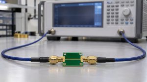
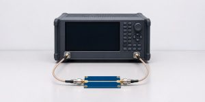
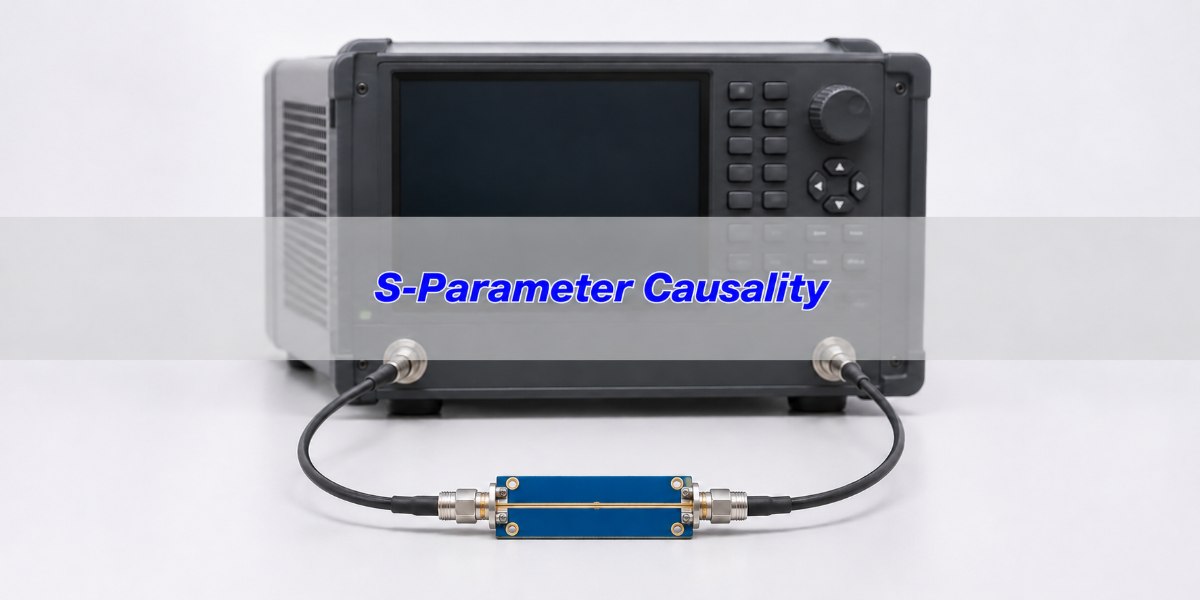
An RF PCB coupon with coaxial connections in front of a network analyzer
Capture the measurement setup and reference planes before comparing transformed or fitted time-domain data.

What Is S-Parameter Causality?

A causal network does not respond to a future input. For a correctly referenced linear time-invariant model, the physical impulse response is zero before the excitation at the input reference plane. For a transmission path a known physical delay can give a more specific expected onset, although estimating it requires the actual path, propagation model and reference planes. A reflection at the calibrated input plane can legitimately begin near zero.

Passivity and reciprocity test different properties. The S-parameter passivity check examines whether a passive model creates net power, not whether it responds too early. A small negative group delay over a limited band is likewise not, by itself, proof of noncausality. Use the full measurement and modelling context, rather than one plot attribute.

S-Parameter Impulse Response: Why a Causal Path Can Show Pre-Ringing

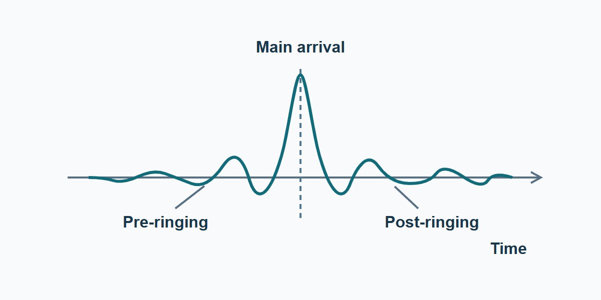
An inverse Fourier transform of a measured sweep works with finite bandwidth. Limiting the spectrum multiplies it by a frequency-domain window; in time this convolves the actual impulse with the window’s time response. A sharp truncation can create sidelobes before and after a causal pulse. A softer window often suppresses sidelobes but broadens the main pulse, so nearby features become harder to separate.

Keep the time origin and original data fixed. Compare the early response with a known line or thru using the same processing and record how it changes under reasonable windows and measured spans. Small features near the main arrival that vary as expected with the window are consistent with truncation. Do not call them real PCB events or declare the file good solely because one strong window hides them.

Illustrative impulse showing sidelobes on both sides of the expected main arrival after band limiting
Schematic only, not measured data. Finite-band processing can put sidelobes ahead of the main arrival without making the real device noncausal.

Frequency Step Size: A Late Echo Can Appear at Negative Time

On a uniformly spaced frequency grid, the inverse-transform time record repeats with period T = 1 ÷ Δf. Span and step do different jobs: a larger measured bandwidth can separate closer events, while a smaller frequency step extends the record. Zero-padding or interpolating the same measured samples does not supply independent frequency points or prove that a late event is inside the measured record. If your solver needs a different frequency grid, use this S-parameter interpolation guide to compare Cartesian and polar methods against withheld measured points.

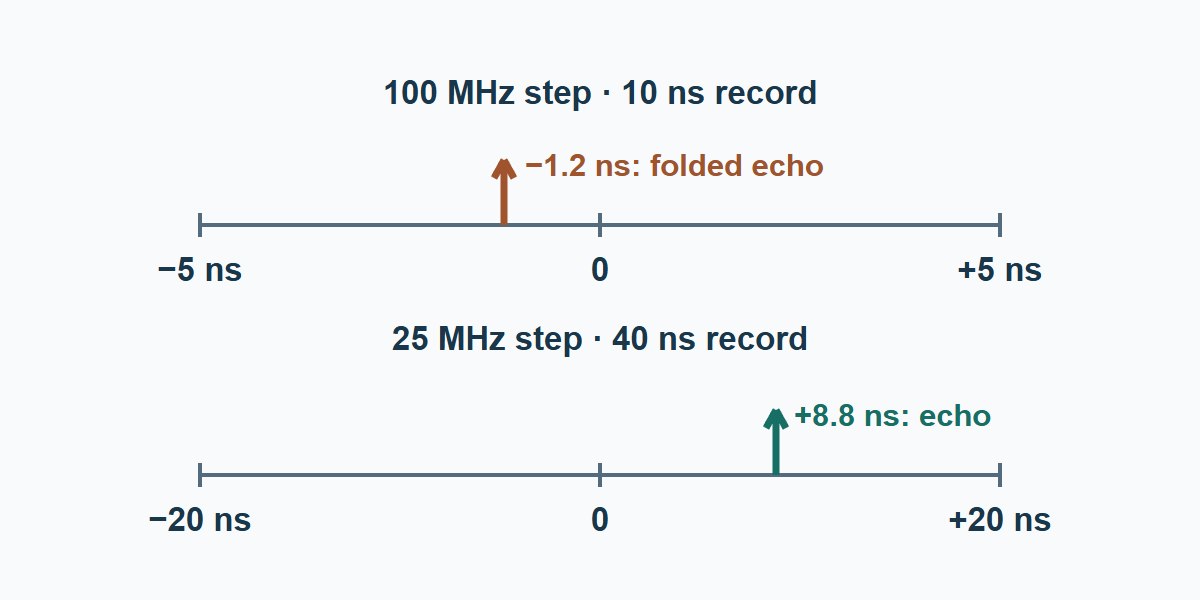
Worked example: assume a delayed echo at +8.8 ns. With a 100 MHz step, T is 10 ns and a centred display covers −5 ns up to +5 ns. The echo appears at 8.8 − 10 = −1.2 ns in that period. Re-measure the same band on a 25 MHz grid and T becomes 40 ns; the centred record goes from −20 ns up to +20 ns and can show the echo at +8.8 ns. These times illustrate ideal periodic mapping, not measured results.

A plus 8.8 nanosecond example echo appears at minus 1.2 nanoseconds in a 10 nanosecond centred period and at its positive time in a 40 nanosecond period
Keep bandwidth comparable and physically reacquire the finer grid. Do not infer additional measured time range from display interpolation.

VNA Time Domain: Three Lookalike Faults and Their Checks

Put separate tests around three questions: does the feature track the frequency window, does it move with the record period, or does it first appear during model processing? Perform the changes on a saved copy and verify instrument calibration on the actual sweep grid. Every new data record needs an identifiable setup and reference.

What you see Check that separates it What the result supports
Small features clustered either side of the main arrival Compare two reasonable windows and a known line at the same reference planes. A change in spacing or sidelobe amplitude consistent with the reference supports a finite-band artifact.
Isolated early pulse Re-measure at the same span with a finer frequency step, keeping the setup comparable. A feature moving by an amount consistent with the repeat period supports a folded response.
Entire response moves after port extension or fixture removal Compare raw and processed stages against a known path and check removed delay and sign. Hold the processed model until time origin and fixture assignment agree.
Early feature persists in a physically implausible location after controlled changes Compare independent reference measurements and validate the model method and settings. Do not dismiss it as ringing; isolate the first failing stage and do not release unverified data.

S-Parameter Reference Plane: Check the Delay You Removed

Keep a sketch from the VNA calibration planes to the DUT planes, with port numbers and the fixture on each side. Compare the untouched sweep with each processed file. On a transmission path a simple delay correction changes phase slope and shifts time. If the applied correction removes more delay than the physical fixture contributes, a correctly measured arrival can appear too early in that processed file.

For example, if an arrival is 1.4 ns from the raw reference and the documented combined fixture delay is 0.6 ns, a delay-only correction would leave about 0.8 ns in this illustrative case. Removing 1.6 ns instead would place it at about −0.2 ns. Real de-embedding can also change amplitude and reflections, so do not treat every fixture as a pure delay. Verify on a reference, and check units and port extensions before editing the DUT model.

If the delay was removed at the instrument, use the VNA port extension guide to check each port’s one-way delay and verify the shifted plane with an independent standard before judging a time-domain arrival.

DC Extrapolation: Use the Physical Low-Frequency Path

A sweep starting above DC does not establish what happens at DC. A through connection with a resistive path and an otherwise isolated series-capacitor path have different low-frequency limits. Use the schematic, DC resistance when relevant, and a suitable low-frequency reference to constrain the extrapolation. Do not assume S21 = 1 or extend the first sample flat for every PCB network.

For a serial interconnect, compare transient results under justified low- and high-frequency continuations, including any actual coupling components. For a DC-blocking filter, use a low-frequency model that preserves the open series path; a convenient flat extrapolation can create a misleading step baseline. In both cases, report which bands were measured and which were estimated. If the outcome changes beyond the project tolerance within plausible assumptions, limit what the model may be used for or remeasure.

Vector Fitting S-Parameters: Compare the Fit With Original Measurements

A well-formed stable, proper rational model with a physically appropriate nonnegative delay can be a useful causal representation. But a fit forces structure on the data. It cannot prove the real PCB matches the result, especially outside the measured band. Do not “fix” a large early pulse by zeroing the response before an arbitrary time; changing the time waveform also changes the frequency response.

For a backplane or cable launch, verify the fit against complex S-parameters, expected delay, and the transient or eye metric used by the system team. For a narrowband RF filter, preserve the wanted passband transmission and phase as well as the stopband range your fixture can establish. For a passive channel, run a separate passivity check on the resulting model and inspect the errors after any enforcement. Reject or limit a fit that meets numerical criteria only by losing a response the application depends on.

S-Parameter Quality Check: What to Sign Off Before Handoff

Use this worksheet when sending a model to a designer or accepting it from a vendor. Fill in the measured band, actual point spacing, reference planes, expected arrival, and the early-time interval used for review. State how acquisition, repeatability and processing affect the decision. There is no universal percentage of pre-arrival energy that applies regardless of bandwidth and window.

Record Evidence to include Action if missing or inconsistent
Measured sweep and origin Device and fixture IDs, planes, grid, settings, and reference device trace. Hold timing comparisons until another engineer can reproduce the origin and band.
Early feature example 100 MHz grid shows −1.2 ns; a qualified 25 MHz remeasurement confirms a corresponding echo at +8.8 ns. Record the original reading as a display wrap candidate. Confirm the actual echo on the extended record before releasing the original timing claim.
Processing and intended use Window, extrapolation, fixture removal, fit method, residuals and intended application and band. Do not generalize the fit to unqualified conditions. Refit, remeasure or set limits on use.

IEEE 370-2020 covers electrical characterization and measured-data quality for printed circuit boards and related interconnects up to 50 GHz. If invoked, apply the agreed method and derived acceptance criteria; the case values above are teaching examples, not IEEE thresholds or PCB workmanship limits.

S-Parameter Causality FAQs

Does every sample before time zero mean a noncausal PCB?

No. Check finite bandwidth, record wrap, reference plane and the measurements before judging the model.

How do I tell ringing from time wrap?

Compare windows on a fixed data set for ringing. Re-measure with a finer frequency step and similar span to test whether an event moves as a folded echo should.

Does a wider span always increase time range?

No. Time-record period is set by frequency step. At fixed point count, a wider span generally increases the step and shortens the record.

Does zero-padding fix missing measurements?

No. It may increase displayed sample density, but does not add information or replace actual low-frequency or finer-grid measurements.

Can a wrong port extension make a response appear early?

Yes. Excess delay removal can shift an arrival too far left. Recheck the fixture map and a known reference before judging the network.

Must the file contain a measured DC sample?

No, but a simulation sensitive to the DC limit needs a physically justified low-frequency continuation and a stated range of validity.

Does a causal fit prove a passive channel model is acceptable?

No. Separately check passivity, complex in-band error, physical delay and performance in the intended circuit.

Should I trim all pre-arrival samples before simulation?

Not as a first step. Find the cause before changing the waveform and verify any processed result against the original complex data.

Technical References

Custom High-Speed PCBs With Stackup and Coupon Review

Have a high-speed PCB build that depends on a trustworthy channel model? Send EBest Circuit your layout files, stackup, target impedance, connector or fixture assumptions and the coupon requirements. Request a fabrication quote and stackup review to define the build and verification scope before ordering.

You may also like