

Two S-parameter files can agree at every measured frequency and still predict different insertion loss between those frequencies. Before you call the PCB lossy, plot the original measured points over the solver trace. If the extra loss appears only between samples, check how the solver interpolated the complex data. In the worked example below, the interpolation mode alone introduces 3.01 dB of apparent extra loss. That is a calculated example, not a measured board result.
What Is S-Parameter Interpolation?
Interpolation estimates a complex S-parameter at a frequency between measured samples. For example, if the VNA recorded S21 at 4.00 and 4.10 GHz, the simulator may need an estimate at 4.05 GHz. S21 describes forward transmission under the file’s reference conditions; it has both magnitude and phase. A trace can therefore look smooth in dB while giving the wrong phase, or have the right phase but predict too much loss.
Keep the original export as the reference. Tag derived files as interpolated, and record the source sweep, target grid, method, port order and reference impedance. Treat guesses beyond the measured band, including a missing DC point, as extrapolation and review them separately. If your next step is to join two verified models, see this guide to cascading S-parameters with interface reflections before adding their losses.
What a Touchstone File Tells You About Interpolation
The Touchstone option line specifies frequency units and data representation. RI stores real and imaginary values; MA stores linear magnitude and angle; DB stores magnitude in dB and angle. These describe how the original points are encoded. They do not guarantee how the simulator fills in gaps. Re-exporting the same samples as RI does not, by itself, select Cartesian interpolation.
For a useful A/B comparison, keep the measured file, reference impedances, ports and target frequency grid fixed. Change only the interpolation setting. Compare both traces at the original points before investigating what they do between them. If they already differ at the original samples, check renormalization, reference-plane changes and any automatic fitting or smoothing.
Linear Interpolation Formula: Why the Midpoint Loses 3.01 dB
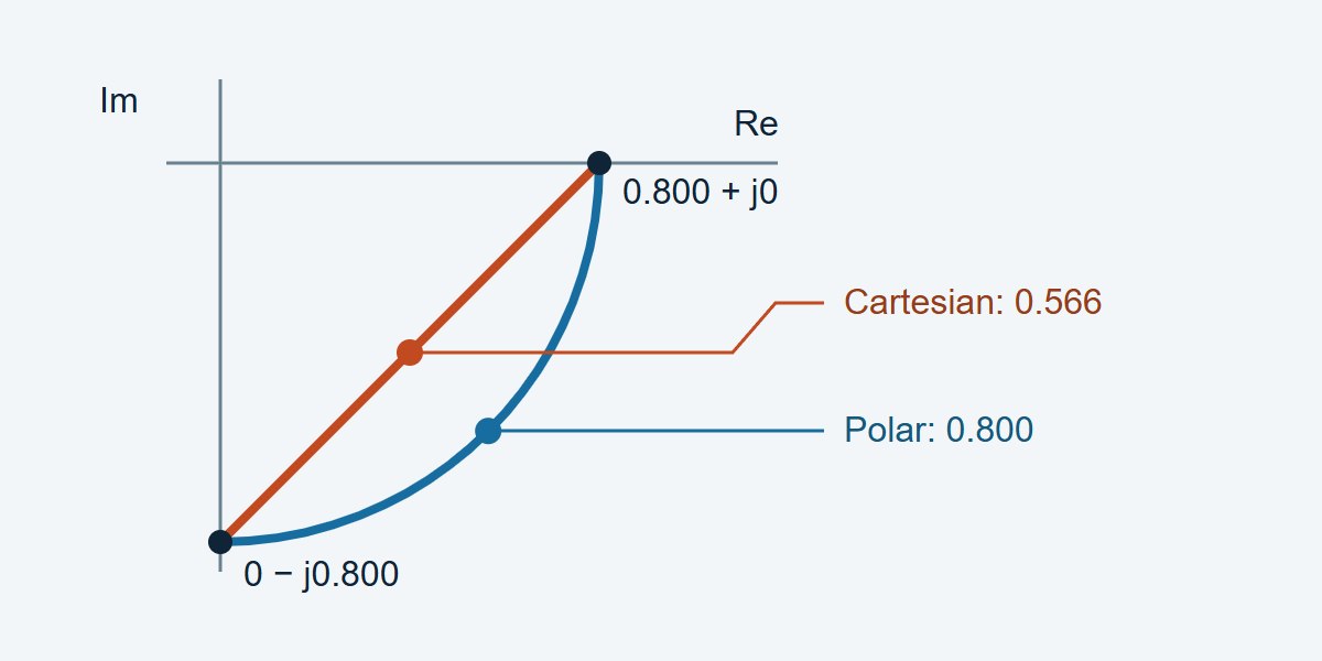
In this calculated example, a path has constant transmission magnitude of 0.800 and delay of 2.5 ns. Between 4.00 and 4.10 GHz its phase rotates 90°. At 4.05 GHz, polar interpolation yields −1.94 dB; Cartesian interpolation yields −4.95 dB. The PCB did not change. The latter method cut across the complex-plane arc.
Let t be the fractional position between the two frequencies. Cartesian interpolation computes (1 − t)S1 + tS2; polar interpolation applies the same weights separately to linear magnitude and unwrapped phase. Here t = 0.5, S1 = 0.800 + j0 and S2 = 0 − j0.800. The Cartesian midpoint is 0.400 − j0.400, with magnitude 0.566. The polar midpoint is 0.800∠−45°. Apply 20 log10|S21| to each magnitude to reproduce the numbers. Insertion loss, stated as a positive loss, is 1.94 dB versus 4.95 dB.
Cartesian vs. Polar S-Parameter Interpolation: Which Should You Use?
Try polar interpolation for a smooth delay-dominated path and test it against measured points you did not give the model. Try Cartesian when the data pass near a null, where phase is difficult to interpret. If the raw sweep missed a narrow feature, neither method deserves a pass until a denser measurement resolves it.
| Method | Try it when | Watch for | Verify with |
|---|---|---|---|
| Cartesian linear (real, imaginary) | Phase becomes unreliable near a null; the complex trajectory is adequately sampled | Chords create loss when phase rotates greatly per step | Midpoint complex residual and S21 loss error |
| Polar linear (magnitude, phase) | Transmission is smooth and delay dominates phase | Phase unwrap can choose the wrong turn; phase near a null is unstable | Measured phase trend, notch depth and ripple |
| Re-measure a finer sweep | A notch, resonance or rapid phase rotation falls between samples | Extra sweep time and drift between passes | Convergence as spacing decreases, with unchanged calibration and fixture |
Phase Unwrapping and Frequency Step Size
A 2.5 ns delay rotates the phase by 90° per 100 MHz, or 180° per 200 MHz. At 180°, a wrapped phase difference alone cannot tell the two directions apart. Even well below that figure, a Cartesian chord can still create unacceptable loss. Near a resonance or deep null, phase can change much faster than the nominal through-path delay suggests.
For a constant-amplitude, constant-delay path, the Cartesian midpoint amplitude ratio is cos(|Δφ|/2) when the actual phase step |Δφ| is below 180°. If the example’s Cartesian midpoint error budget is 0.10 dB, that model gives a maximum step of about 17.36° or 19.3 MHz at 2.5 ns. This is a starting sweep setting for the example, not a VNA specification. Check it with an offset sweep and tighten it where the DUT changes more quickly.
How to Check S-Parameter Interpolation Against Measured Points
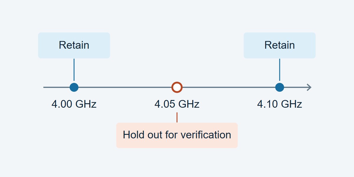
Take a calibrated sweep on a fine grid. Save alternating measured points as a separate verification file, then feed only the retained points to each interpolation method. Compare the predicted results at the withheld points against the saved measurements. Keep VNA settings, fixture, reference planes and signal path unchanged. Repeat near critical frequencies if the measured trace is close to the acceptance limit.
| Check | Record | Decision and next step |
|---|---|---|
| Through loss at 4.05 GHz (example) | Calculated reference −1.94 dB; Cartesian −4.95 dB; residual 3.01 dB | Fails a hypothetical 0.10 dB budget. Try polar, then confirm against an actual held-out sample. |
| Delay-sensitive band | Wrapped phase residual at each held-out point; group-delay residual if required | If outside the design budget, verify phase unwrap and retest with a finer grid. |
| Filter notch or resonance | Measured and predicted feature frequency, depth and critical-band residual | If the fitted shape or frequency fails, measure locally at finer spacing. Near the noise floor, assess uncertainty before classifying depth errors. |
S-Parameter Passivity Check After Interpolation
For a passive network, check passivity over the generated grid, not only at the original points. Where ports use fixed positive real references and power-wave normalization, the largest singular value of the full S-matrix must not exceed one for ideal passive data. An S21 magnitude below one does not prove the network is passive. Evaluate numerical or measurement tolerance separately from the ideal bound.
With a shared linear weight and identical normalizations, Cartesian interpolation of two passive whole matrices preserves the singular-value bound between them. That result does not carry over to arbitrary cubic interpolation, element-wise polar interpolation or causality. For impulse or step simulations, use the solver’s grid requirements and review the S-parameter causality and time-domain checks separately.
S-Parameter Simulation: What to Check Before You Release the File
Channel-loss budget: keep the full band needed for the channel model, identify the frequency or band where spec margin is tightest, and allocate an explicit dB error budget to interpolation. If the residual at an independent point exceeds that budget, do not use the dense model for sign-off.
RF filter model: check that the generated file preserves the passband ripple, stopband rejection and notch location at the frequencies in the filter specification. Add measured points near features rather than relying on a smooth trace or an interpolated null.
Time-domain use: log the measured band and any assumed DC or high-frequency behavior. Repeat the analysis after a finer measurement sweep; compare arrival times and feature amplitudes against the project tolerance, not just the software’s display. Hand off the original file, the derived file and the holdout report together so the next engineer can reproduce the decision.
S-Parameter Interpolation FAQs
Does a denser Touchstone export improve the original measurement?
No. A denser export adds estimates. To establish what the DUT actually did between points, take a finer sweep or independently measure selected frequencies.
Can I interpolate only the dB trace?
For a magnitude-only plot it is a display choice. For a complex simulation, also preserve phase and specify whether the chosen algorithm operates in linear magnitude or dB; these are not equivalent operations.
What phase step is too large?
At 180° the two wrap directions are ambiguous from an isolated pair. Much smaller spacing can already be necessary for your error budget; the equal-amplitude 2.5 ns example needs about 19.3 MHz for a 0.10 dB Cartesian midpoint target.
Can I use polar interpolation across a deep notch?
Only if measurements confirm the result. Phase at very small amplitudes is sensitive to noise, and a coarse sweep may miss the notch depth or position. Re-measure around the feature before deciding.
Should I use a spline instead of a straight line?
Use it only if independent data show that it lowers relevant errors. A smooth spline may overshoot or distort narrow peaks; recheck loss, phase and passivity on the resulting grid.
Is adding a DC point interpolation?
Not unless the measured band already brackets the point. A missing DC value requires a physical low-frequency model, independent measurement, or an explicit extrapolation decision.
Why do two simulators disagree with the same S2P file?
Confirm they use the same ports, reference impedance, reference planes, interpolation domain and out-of-band policy. Then compare their values at the original points and at one withheld midpoint.
Should every S-parameter use the S21 error limit?
No. Set limits for the actual task. A channel model may prioritize forward loss and delay, while a matching problem may require a tight complex reflection error, especially in the bands of interest.
Technical References
- scikit-rf: Network.interpolate — interpolation domains and parameters.
- IBIS Open Forum: Touchstone File Format Specification v2.1 — option line, representations and references.
- scikit-rf: DC Extrapolation for Time Domain — low-frequency assumptions for time-domain use.
Custom High-Speed PCBs With Stackup and Coupon Review
Need custom high-speed or RF PCBs? Ask EBest Circuit to review your proposed stackup and impedance-coupon requirements before fabrication, so you can agree on which layers and structures need to be represented. Send your layout or Gerber files, stackup target, impedance requirements, quantities and requested delivery date to sales@bestpcbs.com for a project review and quotation.
You may also like
Tags: S Parameters, S-parameter causality, S-parameter passivity check, Touchstone file