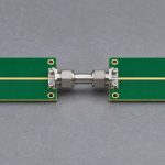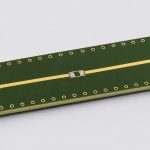


Set the DC limit from the circuit you actually measured, not from the first row of the Touchstone file. A direct copper path and a path with a series DC-blocking capacitor can both look almost lossless at 1 MHz. At 0 Hz, the first still conducts and the second does not. If you copy the first frequency point to DC, a transient simulation can show a voltage that never drains away.
Save the original sweep. Before adding a 0 Hz row or fitting a transient model, identify the circuit and reference planes, calculate the expected DC limit, and test a result that depends on it. If all you need is an in-band RF comparison, leave the unmeasured region unclaimed.
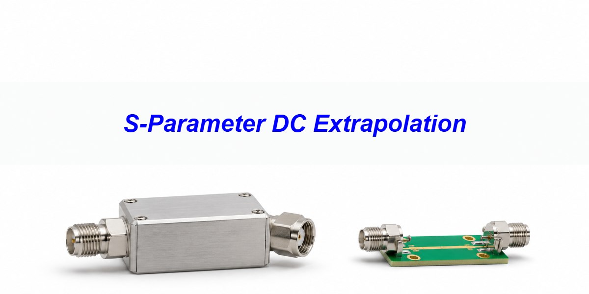
DC Extrapolation: What the Missing Point Controls
DC extrapolation supplies the zero-frequency behavior that a sweep starting above 0 Hz does not measure. In a stable, linear time-invariant system, the DC transfer determines the settled output of a step, provided the simulated source, load, and initial conditions match the intended circuit. It is not a way to recover unmeasured resonances or prove that the fitted transient is accurate.
Use the whole two-port matrix, not just S21. S21 describes forward transmission with port 2 matched to its reference; S11 describes the reflection seen from port 1 under that same condition. A missing match or a simulator load that differs from the reference changes the actual voltage. Start by documenting the file’s reference impedance, physical port map, and whether coupling components and any bias network were included.
S-Parameter DC Extrapolation: Start With the DC Circuit
Draw the circuit between the actual measurement planes. Carry resistances and DC terminations into that drawing; in a first-pass ideal capacitor model, replace each series capacitor with an open. A through path, an isolated series break, and a through path with a shunt to ground have different DC limits. Include real leakage or bias paths if they matter to the system. Resistance between signal pins alone does not establish the shunt paths to ground.
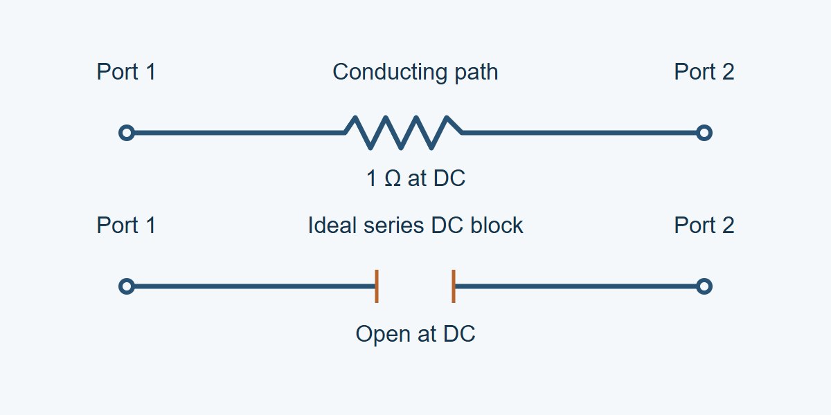
For equal, real 50 Ω reference impedances and one series impedance Z between the ports, S21 = 100 Ω ÷ (100 Ω + Z) and S11 = Z ÷ (100 Ω + Z). A 1 Ω through path gives S21 = 0.9901 (−0.086 dB) and S11 = +0.00990 (about −40.09 dB). An ideal series open gives S21 = 0 and S11 = +1. Keep the latter sign: an open and a short can both have reflection magnitude 1, yet they are not the same circuit. When a measured load is close to an open rather than exactly open, see the VNA high impedance measurement guide for deciding whether the fixture can resolve a finite value.
AC Coupling Capacitor: Why 1 MHz Is Not DC
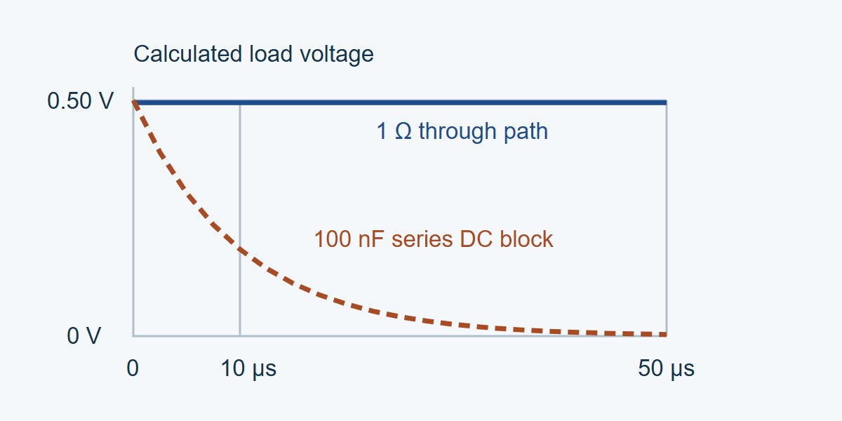
In this calculated example, an ideal 100 nF series capacitor works between a 50 Ω source and a 50 Ω load. Its time constant is (50 + 50) Ω × 100 nF = 10 µs, corresponding to a −3 dB point of roughly 15.9 kHz relative to the high-frequency transmission of this ideal circuit. At 1 MHz the reactance magnitude is about 1.59 Ω and |S21| is 0.99987, or roughly −0.0011 dB. That first measured frequency is well above the corner and cannot identify the DC behavior on its own.
With a 1 V ideal source step ahead of the 50 Ω source resistance, the matched load starts at 0.50 V and decays to 0 V. The ideal load voltage is 0.50 e−t/10 µs V: about 184 mV at 10 µs and 3.37 mV at 50 µs. Compare that with about 0.495 V settled for the separate 1 Ω DC-connected path. These are calculations for simple circuits, not measured board data or recommended global limits. A real dielectric, bias resistor, source waveform, or termination can change the result.
DC Measurement vs. Extrapolation vs. Circuit Modeling
| Method | When to use it | Trade-off and check |
|---|---|---|
| Independent DC and low-frequency measurement | You can access the correct planes and the device remains in its operating state. | Confirm terminations and parasitic effects. A four-wire resistance check can support a simple through path; it does not measure the low-frequency knee or characterize a biased active network. |
| Topology-constrained circuit or fit | The topology is known but the VNA cannot reach the region that controls the transient. | Constrain the DC limit and compare with overlap or separate low-frequency data. Do not add a coupling capacitor again outside the model if it is already inside. |
| Automatic DC extrapolation | Exploratory plots, or a verified near-DC sweep with justified behavior. | Convenient but algorithm-dependent. Inspect the imported zero-frequency matrix and compare against topology and a reference response. Restrict use if those checks fail. |
Touchstone File: Keep the Measured and Derived Files Separate
Archive the original file as measured. Make a separate model identified as DC-extended. Record the original start frequency, point spacing, first measured point, derived DC matrix, reference impedance, and whether the analysis tool resamples onto a uniform grid. Verify the simulator imports 0 Hz as intended; some workflows synthesize their own endpoint or require a particular grid for a low-pass transform. A scope-like time plot is not proof that the software used your DC row.
For a passive real circuit with consistent real port references, a finite zero-frequency matrix should be real. A fit or extrapolation should not introduce gain or an impossible low-frequency shunt. For a cascaded path, check that each section agrees on the interconnection and impedances before assembling it; see cascading S-parameters without losing mismatch information. Keep the component and de-embedding boundaries explicit rather than forcing a through limit on the entire assembly.
Time Domain Step Response: Check the Tail and the Transition
Use a step suited to what you need to verify. For a DC-blocked link, verify that a long pulse decays toward the expected baseline and that the droop during the intended observation window meets the link budget. A stimulus far shorter than 10 µs in the example above can miss much of the decay. If your data is too coarsely spaced to support the duration of the record for an FFT-based transform, collect a suitable sweep or use an independently tested circuit fit; do not treat zero padding as extra measured data.
For a DC-connected coupon, verify the DC drop with an independent resistance or loaded transfer measurement and then check the early transition against a scope or a valid in-band model. For a fixture with a bias tee, match the actual bias-port termination and operating bias and verify the port that is supposed to block DC. A wrong final value points first to the DC path, termination, or simulator settings; an accurate final value with the wrong decay or transition still needs a low-frequency or bandwidth check.
S-Parameter Model Validation: Use a Release Worksheet
Use this worksheet for a model that will feed an eye diagram, step analysis, or a long-pulse check. Set tolerances from the project and the measurement uncertainty, then capture a falsifiable check. A chart label such as “verified” is not a substitute for the topology, target value, and supporting measurement.
| Test | Record or compare | Decision |
|---|---|---|
| DC block: worked example | 100 nF, 50 Ω each side, 1 V source step, export starts at 1 MHz. Ideal load at 50 µs: 3.37 mV. | If the simulator instead predicts a settled voltage near 0.50 V, reject the DC continuation. Inspect the imported matrix and AC coupling topology. |
| Resistive through path | Port IDs, continuity and resistance at the planes, DC matrix, actual source and load. | Investigate any mismatch between measured drop and modeled final value. Check shunt paths as well as series loss. |
| Shape and band fidelity | First measured frequency, independently checked low-frequency points or decay, residual across the original band. | Reject a model that matches either endpoint or measured band but misses the required decay, droop, or transition. |
| Release boundary | Original and derived filenames, limits on frequency, bias, source/load, and time window. | Release only for intended uses supported by those checks. If needed, label it in-band only. |
S-Parameter Simulation: When to Leave DC Unmodeled
If you are comparing insertion loss only from 2 to 8 GHz and the sweep covers that band, a guessed DC row adds no evidence. Keep the decision inside the measured band. If correcting the endpoint changes the predicted eye baseline or long-pulse droop, the result is sensitive to information that the measured band did not provide. Obtain a lower-frequency reference or a verified circuit description before using the model for a pass/fail decision.
No general PCB workmanship criterion specifies the DC entries in a Touchstone file. Use the product’s actual DC and transient requirements. When discussing a board with your fabricator, specify which path they build and where the measurement ends; agree separately on what any coupon or characterization report must demonstrate.
S-Parameter DC Extrapolation FAQs
Is copying the first data point to DC safe?
Only if independent evidence supports a flat continuation and the circuit’s DC limit. A 100 nF series block can look nearly lossless at 1 MHz while transmitting no DC at all.
Can a VNA measure an actual 0 Hz S-parameter point?
A normal RF sweep starts above zero. Some systems offer separate low-frequency or DC characterization modes or a derived endpoint; check the instrument workflow rather than treating a synthesized DC entry as an RF sample.
Should S11 be zero for a series DC block?
No. An ideal series open with no other paths gives a reflection coefficient of +1 at DC in this 50 Ω example. Zero would represent a matched port.
Does zero DC transmission mean there is no output pulse?
No. The output can jump and then decay because a step contains changing voltage as well as a steady component.
What if the designer already modeled the AC coupling capacitor?
Find the measurement planes. If the capacitor is inside both the imported model and the external schematic, remove the duplicate representation or use a correctly de-embedded model.
Can I check a copper through path with a DMM?
Yes, a suitable four-wire measurement can confirm small DC series resistance at the same planes. It does not by itself establish the complete low-frequency two-port response.
Does a correct DC matrix guarantee a correct transient?
No. The decay, transition shape, losses, and timing also depend on the rest of the model and on the source and load.
What should I send with a DC-extended S2P file?
Send the original export, the derived file, the DC assumptions and basis, the reference planes and port impedances, and the independent check that supports its intended use.
Technical References
- scikit-rf: DC Extrapolation for Time Domain — adding a DC point for impulse or step transformations and checking frequency spacing.
- Keysight: Analyzing Data in the Time Domain — DC treatment in an instrument-specific workflow.
- MathWorks: Fit S-Parameters with a Rational Function — fitting and testing a transient model against the source measurements.
Custom RF PCBs With Stackup and Coupon Review
Planning a new RF PCB or evaluating a prototype before production? Ask EBest Circuit to review the proposed stackup, RF transitions, and coupon placement. Reviewing the board layout before quoting gives you a chance to put the measurement planes where they serve the design, instead of leaving them to a last-minute fixture.
Send your layout files, stackup, working band, impedance targets, and quantities to sales@bestpcbs.com. Request a custom RF PCB quote and tell us what the coupon needs to verify.
You may also like
Tags: S Parameters, S-parameter renormalization, Touchstone file