

A low pass filter keeps the slow part of a signal and reduces the faster part. The cutoff tells you where the response starts to roll off; it does not tell you whether the wanted signal survives or the unwanted signal is quiet enough. Check both before choosing a circuit.
Consider an analog sensor whose signal extends to 200 Hz and picks up interference at 20 kHz. A 10 kΩ resistor and a 10 nF capacitor look like a good fit on paper. Connect a 10 kΩ input, though, and the same board loses half its low-frequency voltage. This guide shows how to catch that change before ordering boards and how to verify it on the bench.
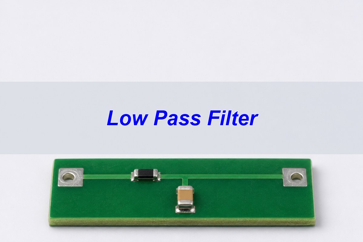
What Is a Low Pass Filter?
A low pass filter passes frequencies below its transition region more readily than frequencies above it. The passband contains signals you want to preserve. The stopband contains signals you want to suppress. Between them, gain changes gradually. It is not a switch that cuts everything above one frequency.
For this sensor, preserving 200 Hz and reducing 20 kHz are separate requirements. In an audio crossover, the same idea sends low notes to the woofer while attenuating higher ones. A filter cannot remove noise that occupies the same frequencies as the useful signal. If the noise is in-band, look at shielding, grounding or the signal source instead of lowering the cutoff until the wanted signal disappears.
How a Low Pass Filter Circuit Works
In a passive RC low pass filter, a resistor sits in series with the signal and a capacitor connects the output node to ground. Measure the output across the capacitor. At DC, the capacitor draws no steady-state current, so an unloaded output follows the input. At higher frequencies, the capacitor’s impedance falls; more AC current returns through it and less output voltage remains.
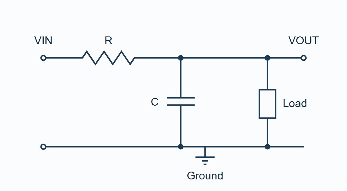
On the PCB, put the shunt capacitor close to the filtered node, with a short return to the intended reference. Keep the unfiltered trace and switching nodes away from the filtered trace; coupling around the resistor gives interference a path the schematic does not show. Leave accessible input, output and nearby ground test points so the lab can check the actual circuit without adding long ground leads.
Calculate the RC Low Pass Filter Cutoff Frequency
10 kΩ and 10 nF give 1.59 kHz with a negligible source resistance and a high-impedance load. With a 10 kΩ resistive load across the output, the cutoff rises to 3.18 kHz relative to its own passband, and the low-frequency gain drops to 0.50 V/V. This is why a board can show the wrong corner even when both fitted components are correct.
For an unloaded first-order network, fc = 1/(2πRC). If source resistance is Rs and the load is RL, use the resistance seen by the capacitor with the ideal source set to zero: RTH = (Rs + R) ∥ RL. Then fc = 1/(2πRTHC). The low-frequency gain from the ideal source is G0 = RL/(Rs + R + RL). This model assumes a linear, resistive load. A switched input, capacitive load or transmission-line termination needs its own model.
| Model input or result | Unloaded | 10 kΩ load |
| Resistance seen by C | 10 kΩ | 5 kΩ |
| Low-frequency gain | 1.00 V/V | 0.50 V/V |
| Cutoff from local passband | 1.59 kHz | 3.18 kHz |
| 20 kHz gain relative to local passband | −22.01 dB | −16.07 dB |
With a ±1% resistor and a ±5% capacitor, the unloaded cutoff spans about 1.50–1.69 kHz using tolerance extremes alone. The calculation does not include changes in capacitance from DC bias, temperature or aging. Use effective capacitance at the operating point where those effects are material.
Specify the Low Pass Filter Frequency Response
Define the response at two points before you pick the components: the highest wanted frequency and the first unwanted frequency that must be suppressed. For this example, allow at most 0.10 dB loss at 200 Hz relative to the passband, require at least 20 dB attenuation at 20 kHz relative to the passband, and separately require at least 0.95 V/V in the passband. These are assumed project limits, not universal acceptance standards.
For one pole, relative gain is −10 log10[1 + (f/fc)²] dB. Solving at both frequencies gives an acceptable cutoff window of about 1.31–2.01 kHz. The unloaded 1.59 kHz design sits inside the window. The loaded 3.18 kHz version does not: it loses useful voltage and suppresses less of the interference relative to what it passes.
If the low end of the cutoff window ends up higher than the high end, no first-order cutoff can meet both limits. Add a pole or change the signal or noise conditions. Simply increasing C solves the stopband at the cost of more loss at the top of the passband.
Low Pass Filter vs High Pass Filter
Use a low pass filter when the useful signal is below the noise; use a high pass filter when the useful signal is above it, for example when removing DC offset from an AC signal. A high pass filter is the wrong choice for a sensor that must retain DC. The same R and C can give the same nominal corner in both topologies, yet they retain opposite ends of the spectrum.
| Circuit | What it keeps | When to use it |
| RC low pass | DC and slow variations | Keep sensor output, reduce high-frequency interference |
| RC high pass | Fast variations; blocks DC | Remove offset before amplifying an AC-only signal |
| Band pass | A frequency band; attenuates both ends | Isolate a tone or modulated signal; not for DC sensing |
When Active Low Pass Filter Design Makes Sense
A passive RC stage is the simplest choice when voltage headroom is limited, the downstream input is high impedance, and one pole meets both limits. If adding the destination input changes the pole or passband gain, a unity-gain buffer is often the next step. If the specifications need a steeper slope or a controlled second-order response, choose a dedicated active stage rather than connecting two identical passive stages and assuming their unloaded responses multiply.
| Topology | Choose it when | Check before committing |
| Passive RC | One pole is enough and the load barely affects it. | Source resistance, downstream input and effective C. |
| RC plus buffer | A single pole works but the next stage would load it. | Buffer common-mode range, output swing, noise and stability with the load. |
| Second-order active | Need steeper rejection or controlled step response at signal level. | Response family, stage Q, amplifier bandwidth and tolerance. |
| Passive LC | Power or RF constraints make resistive loss impractical. | Termination, resonance, damping and component parasitics. |
Butterworth vs Bessel vs Chebyshev vs Elliptic
Start with Butterworth if flat gain matters, Bessel if timing and pulse shape matter, Chebyshev Type I if you can trade passband ripple for stronger rejection, and elliptic (Cauer) if an interferer sits close to the band edge and ripple in both bands is acceptable. These are response families; Sallen–Key is a circuit topology, not a response family.
The calculated comparison below uses ideal fourth-order analog models with the same passband edge: 1 kHz at −0.5 dB relative to peak passband gain. Chebyshev Type I and elliptic use 0.5 dB passband ripple; the elliptic example is designed for 40 dB minimum rejection in its specified stopband. The 2 kHz figures are a comparison at one frequency, not measured specifications or guarantees across the stopband.
| Response | Loss at 2 kHz | Use and check |
| Butterworth | 15.1 dB | Flat gain, no ripple. Check the first unwanted frequency. |
| Bessel | 2.1 dB | Preserves pulse shape. Check delay variation and step settling. |
| Chebyshev Type I | 30.6 dB | Sharper roll-off, with passband ripple. Check ripple and step overshoot. |
| Elliptic (Cauer) | 40.8 dB | Steepest here, with ripple in both bands. Sweep the whole stopband, not just one notch. |
If your example target is at least 30 dB at 2 kHz, Chebyshev Type I and elliptic meet it in the ideal model, but the Chebyshev margin is only 0.6 dB. Check component tolerances, source and load impedances, and op-amp bandwidth before choosing either on that basis. If the circuit instead has a strict delay or overshoot limit, verify that separately with a group-delay sweep or a step test.
Read a Low Pass Filter Bode Plot
At a first-order low pass filter’s cutoff, the output amplitude is 1/√2, or about 70.7%, of its low-frequency passband amplitude. The voltage calculation is 20 log10(0.7071) = −3.01 dB, normally called the −3 dB point. With the same impedance, that amplitude ratio corresponds to half the power. It is 70.7% of the input only if the passband gain is unity.
In the loaded RC example, that same calculation gives 0.50 × 0.7071 ≈ 0.354 V/V at 3.18 kHz. On an input-referenced Bode plot, the passband is −6.02 dB and the cutoff is −9.03 dB. When checking a higher-order response, confirm how its band edge is defined; a specified 0.5 dB ripple edge, for example, is not the −3 dB point.
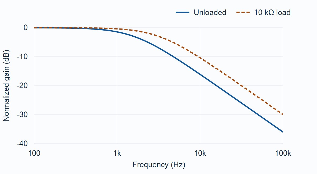
Far past cutoff, one pole approaches −20 dB per decade and two poles approach −40 dB per decade. These are slopes, not promised attenuation values at the edge. Phase matters too: a first-order low pass is −45° at its cutoff. If phase or settling is part of the application, verify it separately; a magnitude plot alone cannot prove a pulse will settle in time.
How to Measure Low Pass Filter Response on a PCB
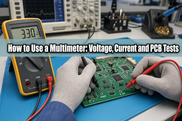
Drive the board with a sine wave, measure the input and output at the same frequency, and record 20 log10(Vout/Vin). Use the same amplitude convention for both channels. Keep the intended load connected for the acceptance run, and record the probe or termination setting. The comparison must use the circuit reference points defined in the test plan, not the generator display.
- Check the setup first. Put both probes on the same low-frequency test node to confirm the channels agree. Check that a scope’s 50 Ω input is not accidentally loading a high-impedance output. Keep signals within the linear range and grounds at the intended reference.
- Measure the low-frequency reference. Record Vin, Vout and passband gain. At 200 Hz and 20 kHz, record absolute gain and then subtract the passband reference to get normalized gain. Sweep around the expected cutoff if the shape or phase is also required.
- Separate the causes. If gain is already low before the roll-off, temporarily disconnect the external load in a controlled bench test. If the passband and pole both recover, check load impedance and consider buffering. If only the pole is off, verify the parts, effective C and probe capacitance. If only the high-frequency rejection fails, check bypass coupling and the instrument noise floor.
- Repeat under the acceptance conditions. Reconnect the specified load and repeat at the same drive, bias, probe, and frequencies. Check absolute gain and both normalized limits before calling the board good. For sampled inputs, use the separate ADC anti-aliasing design guide to set alias rejection rather than assuming this sensor example is the right spec.
Bench worksheet: Use this on a prototype before defining a production test. Enter the actual drive, load, part values, channel settings and measured amplitudes in the test log. The rows below show how to judge readings using the calculated unloaded case; these are not measured results.
| Check | Example result vs limit | If it fails |
| Passband gain | 1.00 V/V vs ≥0.95 V/V: pass | Check the divider and input termination. |
| 200 Hz, relative | −0.07 dB vs ≥−0.10 dB: pass | Check whether the effective cutoff is too low. |
| 20 kHz, relative | −22.01 dB vs ≤−20 dB: pass | Check whether loading shifted the pole. If not, check board coupling and the measurement floor. |
One passing prototype shows that board meets those test conditions. It does not prove every unit passes over component tolerance, supply and temperature. For a build release, agree on what must be checked on each unit and what is covered by design qualification.
Low Pass Filter Applications
The right location and acceptance test depend on what you want to keep: a sensor waveform, an ADC’s measurement band, bass audio, an RF fundamental, or DC power. The following numbers are calculated examples or assumed project limits, not measured results or universal requirements.
Sensor inputs: reduce interference without hiding the signal
Put the RC stage between the sensor output and the receiving amplifier or input. In the bench example above, keep the signal through 200 Hz and reject interference at 20 kHz. With the intended load connected, accept the board only if gain is at least 0.95 V/V in the low-frequency passband, loss at 200 Hz is no more than 0.10 dB relative to that passband, and rejection at 20 kHz is at least 20 dB. If the 10 kΩ load drags the passband down, change the interface or add a buffer before retesting.
ADC anti-aliasing: prevent an out-of-band tone from becoming an in-band error
Put an analog low pass filter before the ADC, taking its driver and input settling requirements into account. At an assumed sample rate of 20 kS/s, interference at 18 kHz folds to 2 kHz. If a 100 mV tone may leave at most 1 mV at the ADC input, allocate at least 40 dB of attenuation at 18 kHz, using the same amplitude convention for both values. Inject the out-of-band tone and check the digitized spectrum at 2 kHz against the calibrated error budget. Also inject an in-band tone to confirm the wanted band still meets its gain limit; repeat at other interferer frequencies the system must handle.
Audio crossover: send bass to the subwoofer without creating a gap
Place an active crossover before the power amplifiers and route the low-pass branch to the subwoofer. For an example 80 Hz fourth-order Linkwitz–Riley crossover, the ideal low branch is about −6.0 dB at 80 Hz and −24.6 dB at 160 Hz, relative to its passband. Check those points in an electrical sweep; they do not prove the speakers sum correctly. Measure the low and high branches together at the intended listening position and check for a dip or peak around 80 Hz against the system’s response tolerance. If the electrical curves pass but the acoustic sum fails, check polarity, delay and placement.
RF output: suppress harmonics without losing the carrier
Place the low pass filter between the RF output stage and its specified load. In an example 50 Ω system, keep a 10 MHz carrier and reduce its 20 MHz second harmonic from −20 to at most −45 dBc. The filter needs at least 25 dB more insertion loss at 20 MHz than at 10 MHz. With the intended terminations, use a calibrated network analyzer to check both frequencies and a spectrum analyzer to verify the final harmonic level at operating power. If the carrier has a separate 1 dB insertion-loss budget, check it independently.
Switching power supply: keep the DC rail while reducing ripple
Where the regulator design permits it, place a damped LC post-filter between the switching supply and the sensitive load. The series inductor opposes fast changes in current; the shunt capacitor gives high-frequency ripple a local return path. If an example requirement is to reduce a 1 MHz ripple component from 20 to 2 mV peak-to-peak, the target is 20 dB attenuation for that component. Compare both sides at the same load and measurement bandwidth, probing at the capacitor pads with a short ground connection. Then step the load and check voltage droop, ringing and settling against the rail’s separate limits. Passing the ripple check alone does not prove the rail is stable under changing load.
Low Pass Filter FAQs
How long does an RC low pass filter take to settle?
An ideal one-pole RC stage reaches about 63% of its final step value in one time constant and 99% in about 4.6 time constants. With unloaded 10 kΩ and 10 nF, that is approximately 100 μs and 460 μs. Check the complete circuit when the output is buffered or sampled.
Can I reduce the resistor and increase the capacitor without changing the cutoff?
Yes, in the unloaded model, if the product RC stays the same. Lower resistance can reduce loading error from the input that follows, but it makes the source drive more current during signal changes. Check the source’s allowed load and the capacitor’s effective value.
Why did adding the oscilloscope probe move the cutoff lower?
Probe capacitance adds to the shunt capacitance. The increase may be negligible at 10 nF but important when the design capacitor is only a few picofarads. Use the probe datasheet, estimate the resulting pole, and verify with a lower-capacitance probe if the shift is significant.
Can I measure the response with a square wave?
A square wave is useful for spotting ringing or measuring settling, because it includes abrupt transitions. Use a sine sweep when you need gain and phase versus frequency. Save both plots when the application has a bandwidth requirement and a separate settling requirement.
Why is the 20 kHz signal still visible after 20 dB of attenuation?
Twenty decibels of attenuation corresponds to one-tenth of the reference voltage at the same impedance conditions, not zero. If 100 mV of interference must drop to 1 mV, you need 40 dB by the voltage ratio. Check that the residual exceeds the test system’s reliable measurement floor.
Can digital filtering replace this analog circuit?
Only if the unwanted content does not already overload the analog input or alias into the sampled band. Once an unwanted signal aliases onto a wanted frequency, a downstream low pass filter cannot distinguish them. Set the analog requirement from the sampling system, then decide how much extra filtering to do digitally.
Will a capacitor across a power rail solve the same kind of noise?
It can lower rail impedance locally, but it acts together with the regulator, interconnect and other capacitors. Do not reuse the sensor RC example to specify a power rail. Check regulator stability, load transients and the frequency of the interference before choosing a rail filter.
Where should I place a low pass filter on a cable-fed sensor board?
Start by identifying where unwanted current enters and where it returns. An entry filter is useful when the interference comes through the cable; a local filter may still be needed at a sensitive amplifier. Keep the dirty and clean traces separate and verify the fitted board with the intended cable connected.
Technical References
- MIT 6.117 lecture 5: first-order filter behavior
- Analog Devices: phase relations in active filters
- Analog Devices AN-649: response families and order selection
- Analog Devices: low-pass response families and elliptic trade-offs
- Texas Instruments: designing active analog filters
- Keysight: Bode plot measurement training kit
- Analog Devices: anti-aliasing filter basics
- Rane: Linkwitz–Riley crossover characteristics
- Analog Devices: measuring switching-supply ripple
Custom PCB Assembly with Engineering DFM Review
Taking an analog board from the bench to a production build? Send your project files to EBest Circuit. A manufacturing review before the build can flag component footprint or assembly risks while you can still change the design. Include the filter test points and acceptance limits if you want to discuss what can be verified on the assembled board.
Email your Gerbers or ODB++, BOM, placement data and target quantity to sales@bestpcbs.com to request a build quote and engineering review.