

PCB manufacturing PCB manufacturing
Home > Blog

RF PCB measurement

S-Parameter Renormalization: From 50 Ω to 75 Ω
Monday, November 16th, 2026

To compare a 50 Ω VNA file with a 75 Ω specification, renormalize the complex S-parameters to the required impedance at the same reference planes. Do not change only the Touchstone header. Renormalization changes how the same electrical network is described. It does not change the actual VNA ports, remove a launch, or repair a poor measurement.

This guide uses linear networks and positive real reference resistances. For complex reference impedances or mixed-mode ports, use a documented method that handles the applicable wave definitions and port mapping.
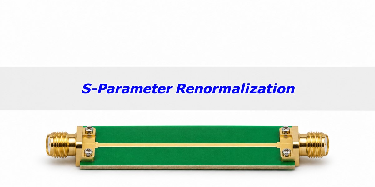
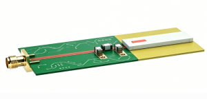
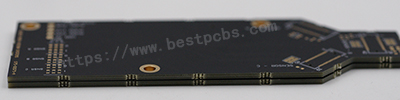
Illustrative RF PCB transmission coupon with coax connectors at both ends
An RF test coupon can be described using different wave references without changing its connectors or the copper geometry.

What Is S-Parameter Renormalization?

S-parameter renormalization expresses the same network at the same physical ports using a different impedance basis for the incident and reflected waves. The voltage-current relationships of the network stay the same; the S-parameter values need not. This is why the same measured circuit can have different return loss under two standards that specify different reference impedances.

Start by recording the original impedance at each port, the port order, the reference plane and the target specification. If the specification calls for a 75 Ω connector-to-connector measurement, a 75 Ω result at the pads is not automatically comparable. Agree on the plane first, not only the impedance number.

Reference Impedance vs. the Physical Termination

The reference impedance is part of the wave definition; a termination is a physical component or a load in a simulation. Changing the reference of a recorded file does not replace the coaxial hardware or change how the source drove the original measurement. If you connect an external load in a simulator, set that load explicitly even when the file is already in the desired reporting basis.

In a two-port S11 reading, the other port is matched to its reference for that S-parameter definition. When you renormalize both ports, that matched condition is different. That is one reason a one-port conversion on S11 alone does not generally reproduce the correct two-port result.

Reflection Coefficient Formula: Check a Known Load First

A known ideal 75 Ω load produces a reflection coefficient of +0.20 in a 50 Ω reference system and zero in a 75 Ω reference system. For a positive real reference resistance R and a load impedance Z, Γ = (Z − R)/(Z + R). The magnitude in dB is 20 log10|Γ|; the positive return-loss convention takes the opposite sign.
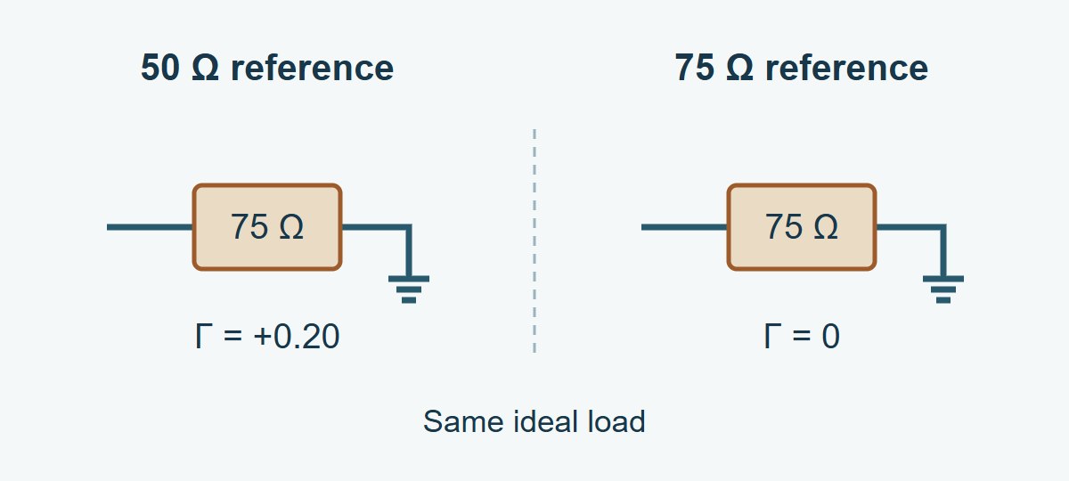
One unchanged ideal 75 ohm load evaluated at 50 and 75 ohm references
In this ideal example the load stays 75 Ω. The reference changes, so the reported reflection changes.

The +0.20 result is −13.98 dB in S11 magnitude, or 13.98 dB return loss. From the original complex Γ, recover the load as Z = R(1 + Γ)/(1 − Γ), then apply the new reference to that same Z. Do not do this from magnitude alone: positive and negative reflections of the same magnitude do not give the same impedance. An ideal open, Γ = +1, makes the finite-Z form singular; use a supported conversion or its limit. A real measured 75 Ω standard will not read exactly zero after conversion.

S21 Measurement: Recalculate the Whole Two-Port

Use a full-matrix renormalization in a tool that supports the file’s wave definition and new per-port values. Do not change only S11 or S22 and leave transmission terms untouched. The result at one port depends on what happens at the other, and complex phase information is part of the data.

Take an ideal 25 Ω series resistor as a check, with the same reference resistance R at both ports. The series current and voltage drop give S11 = 25/(2R + 25) and S21 = 2R/(2R + 25). At 50 Ω, S11 = 0.20 and S21 = 0.80 (−1.94 dB). At 75 Ω, S11 = 1/7 and S21 = 6/7 (−1.34 dB). The reported transmission changed by about 0.60 dB; the resistor did not change. This is an ideal lumped example, not a prediction for a frequency-dependent PCB launch or an uneven pair of port references.

50 Ohm vs. 75 Ohm: Choose the Right Kind of Change

Change the reporting basis only if that is what the problem requires. If the data include a fixture that is not part of the specification, solve the reference-plane problem separately. If the measurement itself cannot resolve the device, improve or verify the physical setup.

What needs to change? Operation What to verify
Wave reference, with the same physical planes Renormalize the full complex network. Correct original and new references; known-load or known-network check.
Location of the reference planes Use a qualified calibration at the new planes or remove a characterized fixture. Which launches remain, and whether the fixture model is valid in band.
Hardware mismatch or usable range Adapt and calibrate the measurement setup as appropriate. Hardware compatibility, matching, repeatability and residual noise.

VNA Port Extension vs. a Reference Impedance Change

Port extension typically compensates for electrical delay and may include loss correction on some instruments. It is not a generic correction for fixture mismatch, and changing R does not move a calibration plane. Verify the instrument’s implementation. If the fixture has appreciable discontinuities or coupling, use an appropriate fixture characterization instead of treating it as a uniform delay.
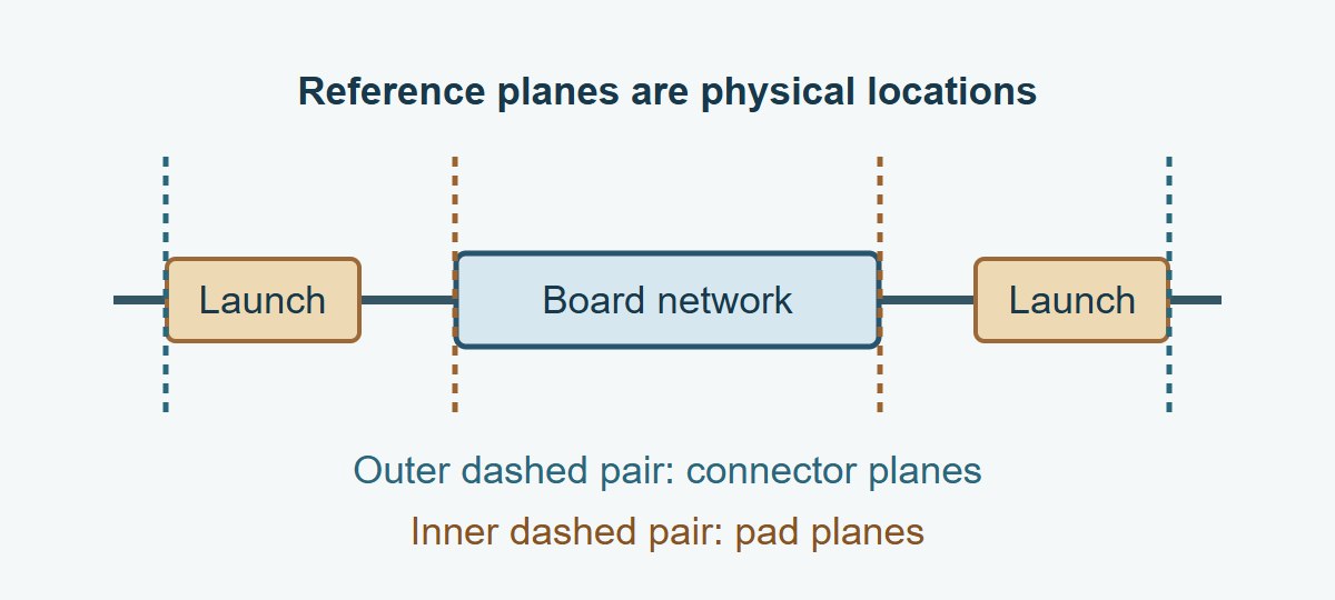
Conceptual measurement path with connectors, launches and distinct connector and pad reference planes
Renormalizing at the connector planes leaves the launches inside the measurement. Moving the planes changes which structure the result describes.

VNA Calibration: Check What the Physical Setup Can Prove

Keep the instrument’s physical ports and its software impedance setting separate. For example, Keysight’s E5080A system-impedance guidance distinguishes its nominally 50 Ω physical ports from a mathematical 75 Ω display reference. It gives a 75 Ω measurement workflow using suitable matching pads and 75 Ω calibration standards. Apply the supported method for your actual analyzer, calibration kit and rated adapters.

If you have a suitable 50 Ω linear measurement, you can convert it mathematically, but conversion does not restore a response missing below the floor or remove unstable coupling. When weak S21 limits the claim, use the VNA IF bandwidth guide to verify receiver noise and fixture leakage before converting or releasing the result.

Touchstone File: Check the Export Before Sending It

Save the original raw file, export a separate converted copy, and reopen it in the receiver’s tool. In Touchstone 2.0 and 2.1, the optional [Reference] keyword supplies port-ordered real reference resistances and overrides the option-line default when present. Touchstone 1.0 uses a single shared reference on the option line; 1.1 has its own per-port syntax. Check importer support rather than relying on the file extension alone.

For a passive PCB channel, use the full-matrix S-parameter passivity check on both versions. Exporting the expected reference values and matching a single transmission trace does not prove the converted data is safe to use in a passive channel model.

Record to check Example entry Pass condition
Physical planes and port order Connector planes; P1 input, P2 output Both versions have the same plane and mapping unless a separate change is documented.
Original and export reference 50/50 Ω → 75/75 Ω Reopened file reports the intended values and transformed complex data.
Known-network check Ideal series 25 Ω: S21 ≈ 0.857 at 75 Ω Use the complex value and expected tolerance, not just the marker after rounding.
Round-trip check Convert the reopened copy back to 50/50 Ω Original complex data are recovered within declared numerical tolerance; this tests software and data handling only.

Use this table for a vendor data handoff. For example, if the exported resistor check still shows S21 = 0.80 while the file shows 75/75 Ω, do not release it: verify that the complex matrix was changed and that the reader recognized the reference format. For a coaxial filter, compare the required return loss and transmission in the specified band at the defined planes. For simulation correlation, verify using the same file reference, frequency grid and actual load definitions. If a change in reference moves the margin around a limit, verify again rather than calling it a physical redesign benefit.

S-Parameter Renormalization FAQs

Can I edit only R 50 to R 75?

No. That changes the metadata without computing the new wave values. Use a valid full-complex conversion and keep the original file.

Can I convert a screenshot that shows S11 in dB?

Not uniquely. You generally need the complex data or both magnitude and phase. Ask for the original file or remeasure.

Does selecting 75 Ω make VNA hardware 75 Ω?

No. A software setting cannot change the physical port construction. Use the instrument’s supported hardware and calibration method when the physical measurement needs to be adapted.

Can ports have different reference resistances?

Yes, when the format and tool support them. Enter the values in the correct port order and verify what the importing program actually applies.

Should I use a different number on the Smith chart after conversion?

Use the chart reference that matches the data and task. A shifted point with a new reference is not evidence that the measured load physically changed.

Does a round trip prove accuracy?

No. It checks conversion and data handling. A measurement can round-trip faithfully and still carry calibration error, noise or fixture leakage.

Can I remove an SMA launch by changing references?

No. Identify the intended plane and use suitable calibration or characterized de-embedding for the launch, independently of the impedance basis.

Do these examples apply to mixed-mode or complex reference data?

Not directly. Define modes, port order and the scattering-wave convention, then use an appropriate documented transformation. This guide uses positive real single-ended references.

Technical References

Custom RF PCBs With Stackup and Test Coupon Review

Send EBest Circuit your stackup, RF connector footprints and test band before release. Reviewing the trace geometry and test coupon together lets your team state which line construction the fabrication check covers and which launches or device responses need separate validation.

Request an RF PCB fabrication quote at sales@bestpcbs.com. Include your released fabrication files, quantity, target impedance by structure, and the required reference planes and reporting conditions.
You may also like

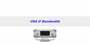
VNA IF Bandwidth: Is Your Filter Stopband Real?
Monday, November 16th, 2026

If a PCB filter’s S21 flattens in the stopband, narrow the VNA IF bandwidth and measure the baseline in the same setup. In a receiver limited by white noise, reducing the bandwidth from 1 kHz to 100 Hz should lower the random noise floor by about 10 dB. If a repeatable plateau remains near the fixture’s isolation baseline, a narrower setting alone will not prove the filter meets its rejection target.

The useful result is not the deepest number the screen displays. It is a reading that can be separated from noise and leakage well enough to decide whether the PCB meets the requirement across the specified band.

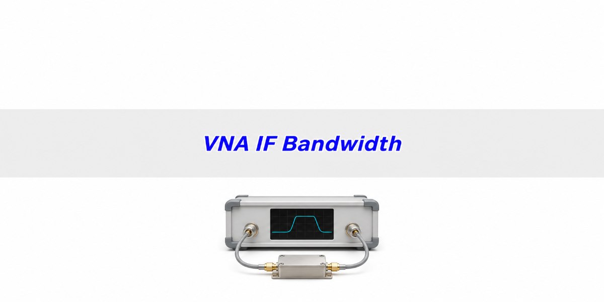
Illustrative two-port vector network analyzer connected to an enclosed RF filter fixture
Illustration of a two-port test arrangement. Keep the physical setup stable while changing receiver settings.

What Is VNA IF Bandwidth?

VNA IF bandwidth is the width of the receiver filter used after the RF signal has been translated to an intermediate frequency. It controls how much noise reaches each measurement point. It is not the RF sweep span, the spacing between frequency points, or the physical bandwidth of the filter under test.

For approximately white receiver noise, noise power is proportional to effective bandwidth. The ideal change is 10 log10(new bandwidth ÷ old bandwidth) dB, so a change from 1 kHz to 100 Hz gives −10 dB. Keysight documents the trend experimentally for one class of instruments. It does not predict the sweep time or lower a signal leaking coherently around the device.

VNA Noise Floor: Check Two Baselines

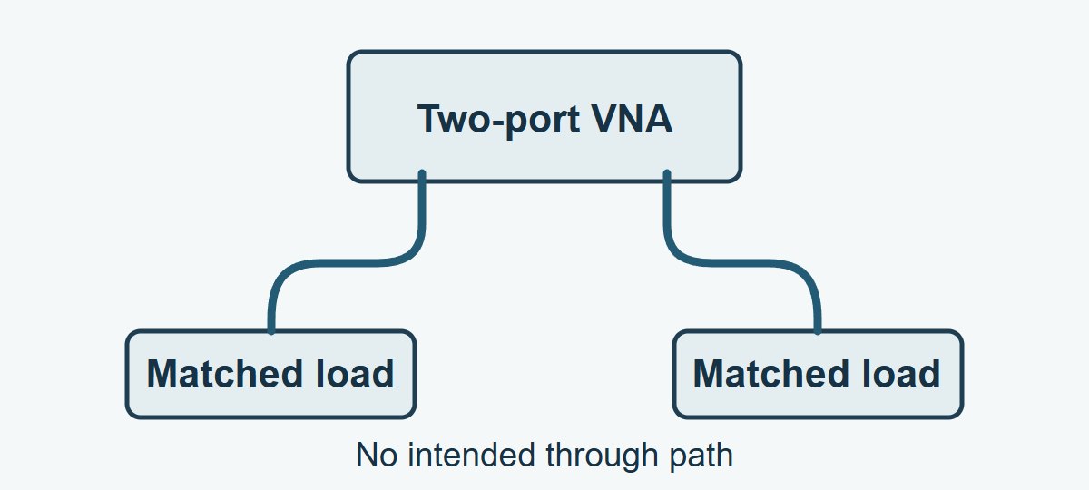
Separate the receiver-and-cable baseline from leakage through the full fixture. A documented isolation check with the two cable ends independently terminated in appropriate matched loads, with no intended through path, shows what the receiver and external setup report under that condition. A representative isolation witness with the relevant fixture retained can reveal coupling that the separately terminated cables missed.

Two independent VNA ports connected to separate matched loads without a through path
Independent terminations are useful for the receiver-and-cable check. Removing the fixture means this check does not capture all of its leakage.

Match source level, receiver mode, frequency grid and IF bandwidth to the device run. Document where calibration ends and whether the analyzer uses isolation correction. An isolation-corrected baseline is not an independent witness if the same trace was used to derive the correction. Follow instrument instructions for appropriate loads and connections. With the real fixture in use, the isolation witness must preserve the geometry and relevant coupling paths; if it cannot, report that limitation.

VNA Dynamic Range: Check the Weakest Part of the Band

Usable dynamic range is set by the actual setup at the frequencies of interest. Check the separation between the device and a relevant baseline point by point, or at the weakest locations under a justified sampling plan. A single best-case dynamic-range number from the front page of an instrument datasheet can miss an in-band leakage spur or a noisier frequency region.

Higher source power can improve a weak reading only while the board and receiver still behave as intended. If the observed gain begins to fall as you raise the drive, use the VNA power sweep guide to check whether the board or the receiver is compressing.

A separation in dB is a screening number, not a measurement uncertainty by itself. Coherent leakage can add or cancel, and receiver noise varies from sweep to sweep. Compare repeats including a reference, and apply the project’s agreed uncertainty and decision rule. If the limit lies within the unverified region, record the measurement limitation instead of assigning a precise stopband value.

S21 Measurement: Record a Wide and a Narrow Sweep

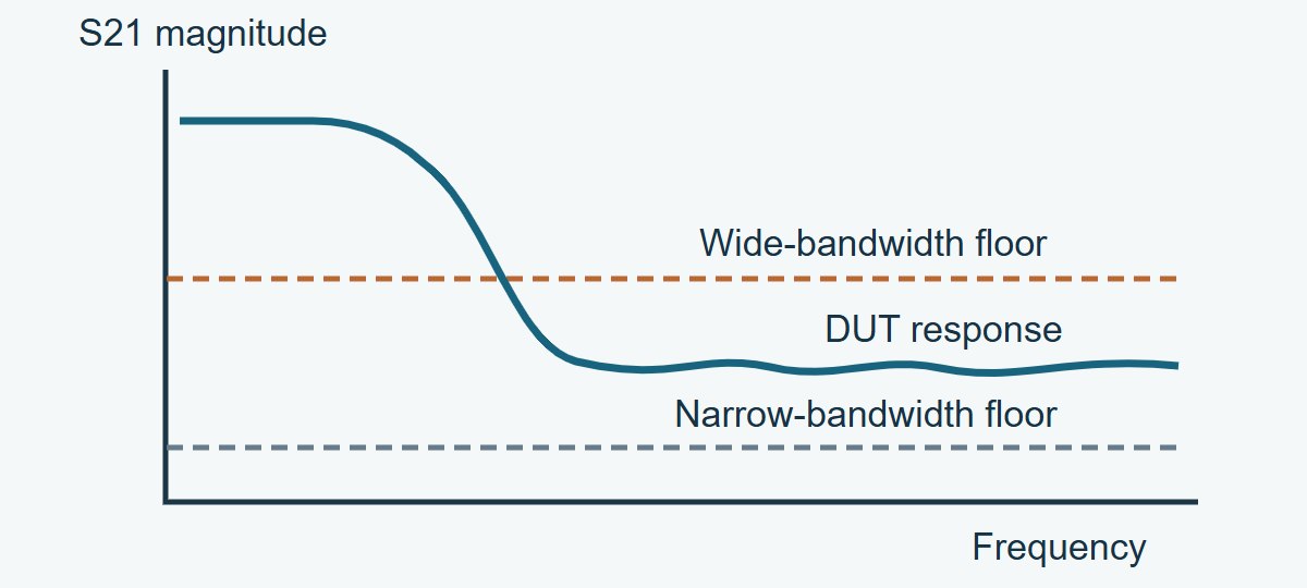
First record the wider-bandwidth baseline, the device and an appropriate reference response. Repeat at a narrower bandwidth with the same grid, test power, fixture geometry and gain settings. Some analyzers adjust operating ranges automatically; verify and record the actual state. Preserve raw sweeps without smoothing. A baseline that drops while the device feature remains repeatable supports a real response. A device trace that drops with the baseline may still be unresolved.

Illustrative S21 plot showing a wide-bandwidth floor partly masking the DUT stopband and a lower narrow-bandwidth floor
Conceptual sketch, not a measurement. Narrowing the receiver bandwidth can separate a DUT response from random noise, but the fixture floor still needs its own check.

Keep the cables still between runs. If a repeatable phase or magnitude change tracks cable pose rather than IF bandwidth, use the VNA cable movement guide to distinguish flex from connector remating. Changing the setting and reconnecting at the same time would obscure which variable caused the difference.

VNA Averaging vs. Narrower IF Bandwidth

Try a narrower IF bandwidth first if the receiver noise is the problem and the sweep budget allows it. Use vector averaging for stable repeated sweeps when you still need better repeatability. Do not substitute trace smoothing for either. Smoothing blends neighboring frequencies and can hide a narrow leak in the stopband.

Control What it changes When to use it
Narrower IF bandwidth Restricts receiver noise per frequency point; usually takes longer to sweep Weak transmission with a baseline that falls when bandwidth is reduced
Vector averaging Combines repeated complex samples; coherent leakage can remain A stable setup where repeated sweeps still show uncorrelated noise
Trace smoothing Combines neighboring frequency points in the displayed response Only for a labeled overview if appropriate; use raw resolution for a narrow-feature limit

For ten independent, equal-weight samples of zero-mean noise, the averaged noise power falls by a factor of ten, or 10 dB. The actual instrument averaging algorithm, settling and drift determine whether its “10” setting behaves that way. Time the completed result, not only the first visible sweep.

VNA Calibration: Recheck It Before Comparing Settings

Set the measurement conditions first where practical, then calibrate to the required reference planes. After an IF bandwidth change, follow the procedure for the specific analyzer. In one Keysight M9485A mode, changing it after calibration can trigger a C-delta status indicating uncertain correction accuracy. Do not assume all instruments handle that change the same way.

Check a suitable reference after the change and recalibrate if the method requires it. Save the correction state, calibration plane, frequency grid, source level and time. If a new calibration changes the reference itself beyond your repeatability allowance, fix or explain that discrepancy before claiming the bandwidth experiment isolated noise.

When comparing a 50 Ω measurement with a 75 Ω requirement, settle the reference basis before interpreting a changed trace. The S-parameter renormalization guide separates mathematical conversion from moving the calibration plane or changing the test hardware.

VNA Sweep Time: Spend Time Where It Changes the Decision

The narrowest setting is not automatically best. Choose the widest validated IF bandwidth that separates the signal from the floor and meets the repeatability needed for your decision. Measure the actual sweep time. Instrument overhead, source changes and filter implementation mean a tenfold reduction in IF bandwidth does not imply exactly ten times the total duration.

On analyzers that support segment sweeps, narrow the receiver bandwidth in the stopband while keeping a suitable frequency grid near narrow features. Keep the rest of the band as fast as the test allows, but verify the full production recipe against a reference. Changing segment boundaries or omitting points to save time must not skip a frequency region covered by the requirement.

Filter Stopband Attenuation: Decide What You Can Report

Use the worksheet below at a defined frequency where a result may be limited by the setup. Enter the absolute S21 display levels at the same conditions and subtract the baseline from the DUT reading. Then decide whether you have sufficient independent evidence for a numerical result. These are teaching numbers; they are not PCB measurements or instrument specifications.

Example condition DUT / baseline, dB Observed separation
1 kHz versus independently terminated baseline −75 / −82 7 dB
100 Hz versus independently terminated baseline −77 / −92 15 dB
100 Hz versus separate fixture isolation witness −77 / −86 9 dB

How to use the third row: subtract −86 dB from −77 dB to get 9 dB. If the contract calls for S21 no higher than −70 dB, the indicated value is 7 dB below that boundary. Neither 7 dB nor 9 dB is the error bound. Check the repeatability, leakage behavior and decision rule before claiming pass. If the isolation witness limits confidence, improve or characterize the fixture rather than reporting extra decimal places.

For a filter stopband, verify frequency coverage, weakest rejection and comparison to the isolation witness. For adjacent PCB paths, retain the relevant routing, launches and return geometry when checking unwanted coupling. For rapid production screening, validate the fastest acceptable setup against a suitable reference and keep a path for retesting borderline samples. Each use case makes a different claim; do not transfer the filter’s measured baseline to a different fixture or board.

VNA IF Bandwidth FAQs

Does IF bandwidth set the spacing between VNA points?

No. Frequency point spacing describes where the response is sampled. IF bandwidth changes the receiver bandwidth at those points. You still need enough points to resolve a narrow feature.

Is averaging dB values the same as vector averaging?

No. Vector averaging works on complex measurements before display; averaging the displayed decibel magnitudes is a different calculation. Use the analyzer’s documented mode and save what it does.

Why does a stable plateau stay at the same level?

It may be real transmission, or it may be repeatable coupling through the setup. Compare the plateau with a suitable isolation witness and change one setup condition at a time.

Can a peak above the baseline still be measurement error?

Yes. A coherent leakage path can add to or cancel real transmission. A repeatable separation supports further measurement, but the setup and the decision rule still determine what can be claimed.

Will changing source power give me more usable range?

It may help in a linear setup limited by receiver noise, but not if the source-to-receiver leakage rises with it or the device enters compression. Stay within equipment and device limits and repeat the baselines.

Can I use a lower IF bandwidth to remove fixture mismatch?

No. It does not correct the impedance discontinuity. Verify the calibration references and treat fixture mismatch separately from receiver noise.

Is the strongest stopband marker enough for a qualification report?

No. Report the weakest relevant rejection across the specified band and any regions where the setup could not establish the requested claim. Keep the original traces and settings.

Should I quote stopband rejection as positive or negative decibels?

Label the convention. An S21 reading of −70 dB corresponds to 70 dB attenuation using the same reference and transmission definition. The direction of the acceptance inequality changes with the convention.

Technical References

Custom RF PCBs With Stackup and Test Coupon Review

Before releasing an RF PCB order, ask EBest Circuit to review the proposed stackup and test coupon requirements together. State the band, target impedances and RF features that must be reproduced so the quote can distinguish board fabrication evidence from the device-level test you plan to run.

For an RF PCB fabrication quote, send your Gerber or ODB++ data, drawing revision, stackup, quantity and test requirements to sales@bestpcbs.com.

You may also like