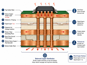


A copper PCB trace becomes more resistive as its conductor temperature rises. If the load current stays constant, its voltage drop and resistive power loss rise as well. A room-temperature resistance calculation is therefore only the starting point for a hot power-distribution path.
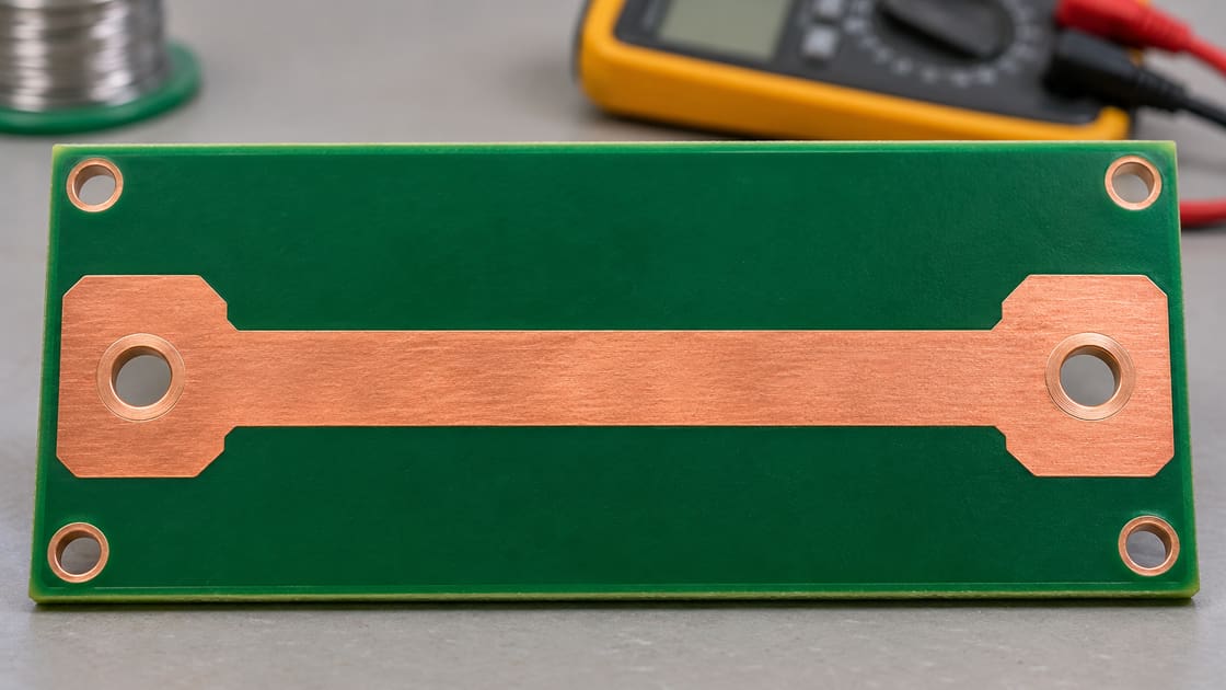
Use this guide to estimate the change and decide what to measure. The worked example describes a uniform trace at a specified temperature; it does not calculate its final operating temperature or establish a current rating.
What does PCB trace resistance describe?
Trace resistance is the opposition a copper path presents to direct current. For a uniform rectangular section, R = rho × L/(w × t), where rho is electrical resistivity, L is length, w is width and t is copper thickness.
Longer paths have more resistance. Wider or thicker paths have less resistance when the other inputs stay equal. This is a DC geometric model: it leaves out connector contacts, vias, local neck-downs and high-frequency effects unless they are separately included. That boundary matters before comparing a calculated trace with a measured complete power route.
Which electrical and geometry inputs are required?
Record conductor dimensions and temperature, not just nominal copper weight. Use consistent units throughout the calculation.
| Input | Unit | Basis used in the teaching example |
| Length L | m | 0.100 |
| Width w | m | 0.002 |
| Thickness t | m | 0.000035 |
| Resistivity at 20°C | Ω·m | 1.68 × 10^-8 |
| Temperature coefficient | 1/°C | 0.00393 at a 20°C reference |
| Conductor temperature | °C | 20 or 80 |
| Constant load current | A | 5 |
The material constants are the approximate copper values used in TI’s FPD-Link ADAS Power-Over-Coax Design Guidelines, section 3.3. The dimensions and operating points are hypothetical. Actual finished copper geometry and material properties can differ; none of these entries is a manufacturing guarantee or a safe-current recommendation.
Calculate the cold resistance first
The hypothetical 100 mm long, 2 mm wide, 35 µm thick uniform trace has a 20°C resistance of 0.024 Ω, or 24 mΩ. Its cross-sectional area is 0.002 × 0.000035 = 0.00000007 m², and 1.68 × 10^-8 × 0.100 divided by that area gives the result.
At a constant 5 A, V = I × R gives 0.120 V across this trace. P = I² × R gives 0.600 W of electrical loss. Those are calculated values for this section alone. They exclude its return path and all other series elements.
Apply the temperature correction to the copper
Use the approximate linear relationship R(T) = R20 × [1 + alpha × (T − 20°C)]. For 80°C copper and alpha = 0.00393/°C, the multiplier is 1.2358, so 24 mΩ becomes about 29.66 mΩ.
The reference temperature belongs to the coefficient and resistance data; do not silently substitute a resistance measured at a different temperature. TI presents this correction for the PCB portion of its example system. For materials, alloys or temperatures outside the intended approximation, obtain the appropriate data rather than treating one copper coefficient as universal.
Compare cold and hot voltage drop at the same current
At a fixed 5 A, the hypothetical 80°C trace drops about 0.148 V and dissipates about 0.741 W. Both are approximately 23.6% higher than their 20°C values because the current is held constant.
| Condition or change | Trace resistance | Drop at 5 A |
| Original geometry, 20°C | 24.00 mΩ | 0.120 V |
| Original geometry, 80°C | 29.66 mΩ | 0.148 V |
| Twice the width, 80°C | 14.83 mΩ | 0.074 V |
| Half the length, 80°C | 14.83 mΩ | 0.074 V |
| Twice the thickness, 80°C | 14.83 mΩ | 0.074 V |
The last three rows hold conductor temperature at 80°C to isolate geometry. They do not predict the new equilibrium temperature or imply equal fabrication cost, routing space or thermal behavior.
Why conductor temperature is not ambient temperature
The copper can be warmer than the air surrounding the board because it dissipates energy and exchanges heat with components, nearby copper and cooling structures. Entering ambient temperature into the correction is valid only if it represents the conductor closely enough for the intended estimate.
For a board inside a closed enclosure, the air itself can differ from the laboratory room. Measure or model the relevant conductor condition under the intended load. A datasheet’s maximum material temperature, a chosen temperature rise and an observed copper temperature are three different inputs, not interchangeable labels.
Include the return path and other series elements
A load sees the voltage available between its supply and return terminals. That depends on the whole current loop, not only the positive trace. Add the relevant return conductor, vias, connectors, protection devices and joints with their own appropriate resistance models.
If the example had an identical return trace at the same 80°C and current, the two copper traces together would drop about 0.297 V. That remains an illustrative copper-only subtotal. Do not apply the copper temperature coefficient automatically to semiconductor switches or contacts, whose behavior requires different data.
Handle neck-downs and changing cross sections
Divide a varying route into sections and add their resistances. A wide pour connected through a narrow segment does not have the resistance of the wide pour over its full length.
Use each segment’s relevant width, thickness and temperature. If current spreads through a large irregular plane, a simple one-dimensional rectangle may be inadequate. The BestPCBs trace neck-down guide discusses the associated local heating risk. Do not average a narrow bottleneck away by substituting the route’s widest width.
Separate electrical loss from the thermal solution
Calculating I²R tells you heat generation at the stated current and resistance. It does not tell you the final temperature without the thermal path. Temperature changes resistance, and resistance changes heating, so the electrical and thermal calculations are coupled.
A useful design process starts with an estimated temperature, evaluates loss and then checks the resulting temperature using an appropriate thermal model or measurement. Iterate as necessary. Do not use the example’s assumed 80°C as evidence that this trace will settle there, or that its surroundings can safely tolerate it.
Check how the load responds to falling voltage
The constant-current example does not describe every load. A regulated downstream converter serving approximately constant power can draw more input current as its input voltage falls, while a simple resistive load behaves differently.
Use the real load characteristic and input-voltage limits. Recalculate the operating point when route loss changes the load current materially. Startup, load steps and undervoltage behavior may also govern the design. The right question is not only “what is the trace resistance?” but “what current and voltage does this complete system reach under the required conditions?”
Verify small resistance without measuring the test leads
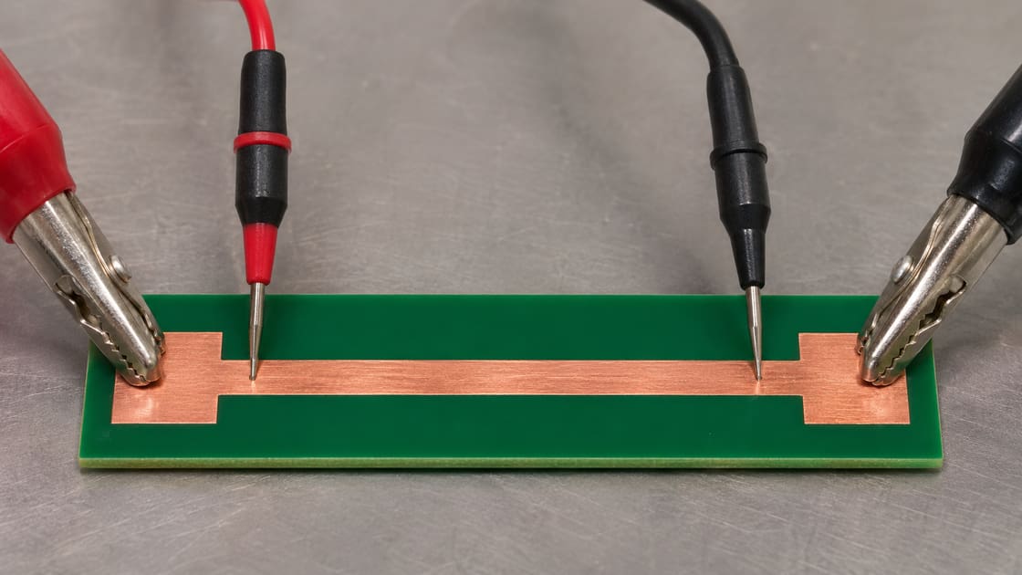
Use an appropriate low-resistance measurement method and defined endpoints. A four-wire arrangement separates current injection from voltage sensing, reducing the influence of lead resistance on the sensed voltage. It does not remove errors caused by incorrect probe locations or an unintended parallel path.
Measure an isolated route or account for the rest of the circuit. Record current, polarity, settling and temperature; test current itself can warm the coupon. Follow instrument limits and safe test procedures. A continuity beep is not a quantitative milliohm measurement or evidence of adequate voltage at the operating load.
Release the power route against a voltage budget
Allocate the allowed distribution drop from source to load, then verify the copper and other series elements under the relevant operating conditions. Check both the cold model and hot evidence, including the return path.
Preserve the finished copper requirement, geometry, current waveform, measurement endpoints and thermal conditions. Choose wider, shorter or thicker routing on that basis, not from copper weight alone. For a Best Technology review, send those inputs and the required load voltage to sales@bestpcbs.com. Manufacturing review does not replace complete-system thermal and electrical validation.
FAQ
Is trace resistance the same as trace impedance?
No. DC resistance describes resistive opposition in the stated path. Transmission-line impedance also depends on geometry, reference conductors and frequency-dependent behavior. A 50-ohm RF trace is not normally a 50-ohm DC resistor. Use the electrical model that matches the measurement and signal or power problem being investigated.
Can I convert a resistance measured at 25°C using the 20°C formula?
Do not treat the 25°C reading as R20. First relate it to the stated reference using the same applicable approximation, or use a coefficient and reference formulation appropriate to that measurement. Record the actual conductor temperature so the comparison does not hide a systematic reference-temperature error.
Does doubling copper weight guarantee half the measured route resistance?
Not for the entire route. The simple model halves resistance only when the actual trace thickness doubles and other relevant inputs remain equal. Vias, contacts, neck-downs, temperature and finished copper variation can prevent the complete path from following that ratio. Compare the same endpoints and operating conditions.
Can I use voltage drop to infer conductor temperature?
Only with a sufficiently characterized path, current measurement and resistance-versus-temperature relationship. Contacts, parallel current paths and nonuniform temperature can distort the inference. For a complex route, resistance represents a combined response rather than one guaranteed local hot-spot temperature. Validate the method before using it for protection decisions.
Why does my multimeter disagree with the geometric calculation?
Check units, actual copper thickness, etched shape, probe endpoints, temperature and parallel connections first. Lead and contact resistance can dominate a small trace value in a two-wire measurement. A discrepancy is not automatic evidence of bad copper; isolate the measured object before assigning a manufacturing cause.
Does low DC voltage drop prove that a power path handles a fast load step?
No. Fast behavior also depends on inductance, capacitance, regulator response and distribution geometry. A route can have low DC resistance yet show a transient voltage excursion. Check the time-domain requirement separately and do not use this uniform DC trace calculation as a power-integrity qualification.
Can I use a standard copper coefficient for a copper-alloy busbar?
Not without verifying the alloy’s properties. Its resistivity and temperature behavior can differ from the pure-copper approximation used here, and joints add their own behavior. Use the material supplier’s relevant data and the complete connection geometry rather than transferring one coefficient based only on the word copper.
Is adding solder a predictable substitute for a wider copper route?
Not by itself. Solder geometry and material properties differ from the finished copper trace, and the resulting cross section can be uneven. A controlled design change requires characterized electrical and manufacturing evidence. Do not assume an informal solder layer delivers a specified resistance, temperature rise or repeatable current capability.