

Noise figure tells you how much a device or receiver chain degrades signal-to-noise ratio under defined conditions. Gain alone does not answer that question. Two RF chains can have the same total gain but different noise figures because the order of loss and amplification matters.
Start with frequency, bandwidth, reference plane and operating state. Then calculate the chain in linear units and measure it with a calibrated method. This guide works through a filter-and-amplifier example, explains Y-factor measurement and shows which missing report fields should stop an acceptance decision.
Noise figure definition: what happens to SNR?
Noise factor F is the ratio of input signal-to-noise ratio to output signal-to-noise ratio, using the appropriate reference conditions. Noise figure NF expresses that factor in dB. It describes added noise relative to the reference source, not simply the output noise level.
An amplifier can produce a larger output signal while still degrading SNR. It amplifies input noise as well as signal, and adds noise of its own. Conversely, a receiver with low output noise is not necessarily sensitive if it has also attenuated the wanted signal.
The standard reference temperature commonly used for RF noise figure is 290 K. State the frequency, gain setting, bias and source/load conditions with the result. A typical specification at one operating point is not a guaranteed value across every frequency or gain mode.
Noise figure vs noise factor: use the right units
NF = 10 log10(F), and F = 10NF/10. F is a linear power-related ratio; NF is logarithmic. For example, 2 dB corresponds to F ≈ 1.585—not a linear factor of 2.
| Quantity | Meaning | Calculation rule |
| Noise factor F | Linear SNR-degradation ratio | Use in the cascade equation |
| Noise figure NF | 10 log10(F), in dB | Convert to linear before cascading |
| Power gain G | Linear power ratio for the applicable chain model | Do not substitute voltage gain or a dB number |
| Output noise power | Noise in a stated bandwidth at the output | Needs gain, bandwidth and source conditions to interpret |
Do not add every stage’s NF in dB. A matched passive loss at the reference temperature before an amplifier is a useful special case; a general cascade requires the gains as well as the noise factors.
Noise figure formula: connect it to a receiver budget
At approximately 290 K, available thermal noise is about −174 dBm/Hz. For a receiver model with equivalent noise bandwidth B in hertz, the input-referred noise level is approximately:
Nin = −174 + 10 log10(B) + NF, in dBm.
Add the required SNR to estimate a theoretical input-signal threshold. Use equivalent noise bandwidth, not an arbitrary spectrum-analyzer resolution setting or a channel label whose filtering has not been considered.
This is not a complete sensitivity guarantee. Modulation, error-rate criteria, implementation loss, interference, gain state and the actual thermal environment can matter. A filter may improve a system’s rejection of out-of-band interference even while its in-band insertion loss worsens the receiver’s noise figure. Those are different effects, not a contradiction.
Noise figure to noise temperature: keep the reference clear
Equivalent input noise temperature is Te = (F − 1)T0, with T0 = 290 K in this convention. It represents the input-referred added noise, not the physical temperature you would measure on an amplifier package.
For a matched passive loss at 290 K, its noise factor equals its linear loss. Thus a 2 dB passive loss has a 2 dB noise figure under those conditions. That convenient relationship should not be applied blindly to a different physical temperature, a mismatched path or an active circuit.
Keep the temperature and reference plane in the budget. A cable before the DUT and a cable after a high-gain DUT do not contribute in the same way to the input-referred result.
Cascaded noise figure: filter before or after the LNA?
For the defined, matched linear two-port model used here, the three-stage Friis equation is:
Ftotal = F1 + (F2 − 1)/G1 + (F3 − 1)/(G1G2).
Use linear factors and power gains. The first stage directly sets part of the result; preceding gain reduces the input-referred contribution of later stages. This is why loss before low-noise amplification can be expensive.
Hypothetical same-frequency components: a matched filter has 2 dB insertion loss at 290 K; an LNA has 2 dB NF and 15 dB gain; the following amplifier has 6 dB NF and 10 dB gain. Assume matched interfaces and small-signal operation, with no mixer or frequency conversion in the example.
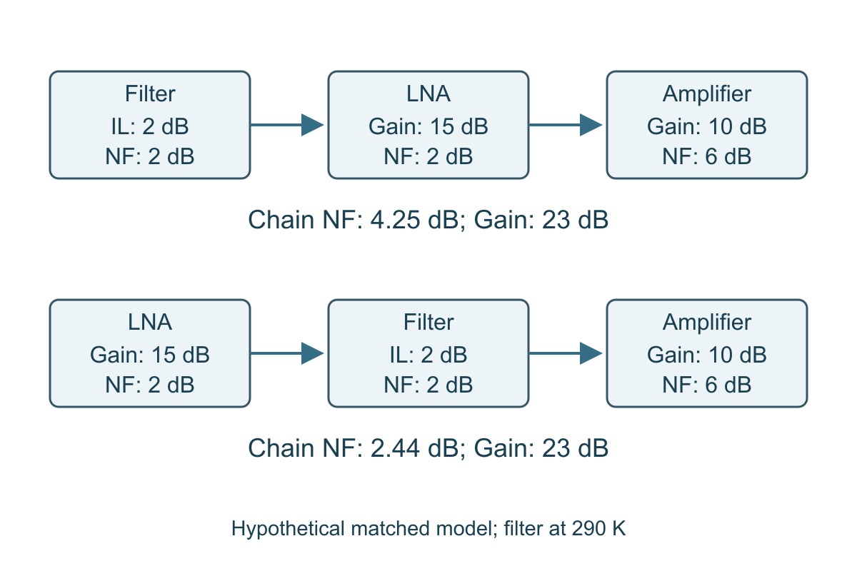
| Same components and frequency | Filter → LNA → amplifier | LNA → filter → amplifier |
| Total power gain | 23 dB | 23 dB |
| Calculated total noise factor | 2.6613 | 1.7528 |
| Calculated NF | 4.25 dB | 2.44 dB |
| Noise-only advantage | Input filtering costs in-band sensitivity in this model | Gain precedes the filter loss |
| Separate decision needed | Whether the filter sufficiently protects against the relevant interference | Whether the unfiltered LNA remains linear under the required blockers |
To reproduce the first column, use filter F = 1.5849 and G = 0.6310, LNA F = 1.5849 and G = 31.6228, and final amplifier F = 3.9811. Calculate Ftotal in linear units, then take 10 log10. Do not substitute “2, 15 and 6” directly into the equation.
With a hypothetical 200 kHz noise bandwidth and 10 dB required SNR, the corresponding theoretical input thresholds are approximately −106.74 dBm and −108.55 dBm, using the rounded −174 dBm/Hz thermal reference. These numbers exclude interference and other implementation losses. The lower-NF option is not automatically the better complete receiver.
Noise figure measurement: how the Y-factor method works
A calibrated noise source provides two known noise states. Measure output noise power in each state; their linear ratio is Y. Under an idealized model with a 290 K cold state and appropriate calibration, F = ENRlinear / (Ylinear − 1).
Calculation example: ENR = 15 dB gives 31.6228 linearly. If the hot/cold output-power ratio is Y = 10, then F = 31.6228 / 9 = 3.5136, and NF ≈ 5.46 dB. Both ENR and Y must be converted correctly; 15 divided by a dB reading is not this equation.
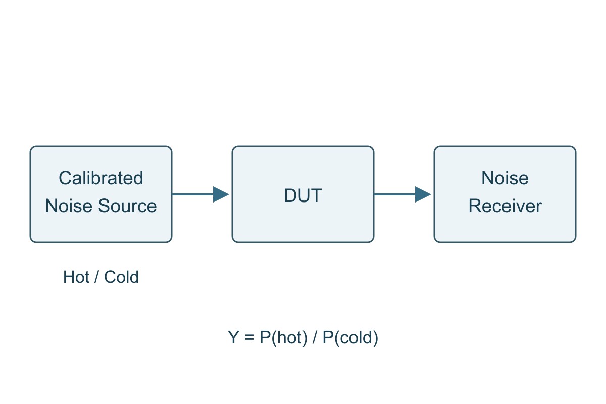
The simple example is not a substitute for instrument calibration. Use the noise source’s ENR data at the actual frequency, account for source temperature and losses, and correct the measurement receiver’s contribution as required. Check DUT bias, gain state, input matching and linearity. A hot noise state that changes gain or causes compression invalidates the constant-gain assumption.
When the measurement plane is moved by a cable, adapter or fixture, update the calibration or loss treatment. Do not subtract an arbitrary cable-loss number from the final NF without following the applicable method and reference-plane convention.
Noise figure in applications: choose the right acceptance test
Weak-signal receiver front ends
Place the noise budget at the actual receiver input, including required switches, filters and feed loss. The worked example shows the sensitivity cost of pre-LNA loss; the design must also survive the expected interference. Verify NF and gain across the band, then verify sensitivity and blocker behavior in the intended gain states.
Do not diagnose every weak link as receiver NF. Antenna radiation and matching are separate contributors; the antenna efficiency guide explains that distinction. Good antenna efficiency does not prove a quiet receiver, and a low-NF receiver does not repair antenna loss.
RF measurement chains
A preamplifier can reduce the input-referred influence of a noisier downstream receiver. It also changes overload margin and may add its own spurs or distortion. Calculate the noise chain with the actual preceding loss and gain, then verify the measurement floor and linear range with the same cables, attenuation and bandwidth used for the DUT.
The acceptance condition is not simply “the displayed floor went down.” The chain must resolve the required signal without compression or an unaccounted calibration change.
Frequency-converting receivers
Mixer specifications need additional care: single-sideband and double-sideband noise conventions are not interchangeable. Image response, conversion gain and following stages affect the interpretation. Do not insert an unexplained mixer NF into the same-frequency example above.
Use the device’s defined noise convention and the receiver architecture, then verify at the relevant RF, LO and IF settings. LO-related noise can also degrade performance through a different mechanism; see the phase noise guide rather than treating all receiver noise as one scalar NF.
Reducing noise figure: balance loss, gain and linear range
First identify loss before the first useful gain stage. Check the intended filter, switch, connector and PCB path at the actual frequency. A short trace is not automatically negligible at every frequency, and a nominally identical connector chain can have different measured loss or mismatch.
Next, assess whether first-stage gain is sufficient to control later contributions. More gain is not free: it can reduce headroom under strong signals. Choose the lowest practical input loss and an appropriate first stage while retaining required filtering and blocker tolerance.
Validate each change in both the noise and large-signal tests. If moving a filter improves small-signal NF but the receiver now compresses under the required interferer, the system is not improved for that application. Record the trade-off rather than selecting the smallest NF number in isolation.
Noise figure report checklist: what can the result prove?
| Report item | Evidence needed | Decision if absent |
| DUT and operating state | Revision, frequency, bias, gain mode and relevant temperature conditions | Do not apply one configuration’s result to another |
| Reference plane | Included cables, adapters and input losses, with calibration treatment | Hold comparisons until the boundaries match |
| Measurement method | Source ENR data, calibration, receiver correction and applicable bandwidth | Ask which assumptions support the reported result |
| Uncertainty and limit | Relevant measurement uncertainty and agreed acceptance rule | Do not invent a guard band or accept a marginal result without a rule |
| System scope | Separate gain, sensitivity, linearity and blocker tests where required | Do not call NF alone a complete receiver pass |
Example review: a report says “NF 2.4 dB” but does not identify the input cable or gain setting. Mark the comparison hold. Request the reference plane and operating state, then compare with the requirement under matching conditions. If the design limit is close to the measured value, resolve uncertainty and the agreed acceptance rule before release.
A bare PCB manufacturing inspection cannot establish the noise figure of a populated RF chain. Specify the RF functional test separately from fabrication and assembly acceptance, and retain the report for the actual assembled configuration.
Noise Figure FAQs
Is a lower noise figure generally better?
For matched frequency and operating conditions, lower NF means less SNR degradation. The complete design must still meet gain, linearity and interference requirements.
Is noise factor the same numerical value as noise figure?
No. F is linear and NF = 10 log10(F). A 2 dB NF corresponds to F ≈ 1.585.
Can I add the noise figures of all stages in dB?
Not generally. Convert to linear noise factors and power gains, apply the appropriate cascade model, then convert the total back to dB.
Why does an input filter worsen NF but sometimes help reception?
Its in-band loss can worsen NF while its out-of-band rejection protects the receiver from interference or overload. Assess both effects in the required test conditions.
What did the equal-gain example demonstrate?
Both modeled chains have 23 dB gain, but moving the 2 dB filter changes calculated NF from 4.25 to 2.44 dB. These are hypothetical small-signal results, not measured receiver specifications.
What does 15 dB ENR and Y = 10 give?
Under the stated ideal 290 K cold-source model, F = 31.6228 / 9 = 3.5136 and NF ≈ 5.46 dB. Real measurements require the appropriate calibration and corrections.
Does −174 dBm/Hz apply at every physical temperature?
No. It is an approximate thermal reference near 290 K. Noise power depends on temperature and equivalent noise bandwidth.
Does NF alone establish receiver sensitivity?
No. Bandwidth, required SNR or error-rate criterion, implementation losses and interference conditions also matter. Verify the actual system requirement.
Technical References
- Analog Devices: system noise-figure analysis — cascade and noise-convention context.
- Analog Devices: measurement methods and formulas — Y-factor relationships.
- Keysight N9069C measurement guide — source ENR, calibration and measurement.
- Keysight: Y-factor measurement accuracy — measurement limitations and uncertainty.
- Rohde & Schwarz: receiver performance — noise, bandwidth and sensitivity.
- Mini-Circuits AN70-001 — input attenuation and mismatch trade-offs.
- Analog Devices: external LNA and receiver sensitivity — system-level use of added gain.
Custom RF PCB Manufacturing with Prototype and Assembly Support
Developing an RF front end or amplifier board? EBest Circuit supports custom RF PCB fabrication, prototypes and PCB assembly. Review the material, stackup, controlled geometry and assembly requirements together so the manufactured board matches the approved RF design and the quoted scope is clear.
Send your fabrication files, material requirements, stackup, impedance targets and quantity to sales@bestpcbs.com for a quotation. Add the BOM and placement data for PCBA. If the project needs gain, noise-figure or other RF functional tests, identify the required method and limits so that scope can be evaluated explicitly rather than assumed from a bare-board inspection.